 LWDAQ User Manual
© 2004-2021 Kevan Hashemi, Brandeis University© 2021-2024 Kevan Hashemi, Open Source Instruments Inc.
| Linux | MacOS | Raspbian | Windows |
| BCAM | Camera | Diagnostic | Dosimeter | |
| Flowmeter | Gauge | Inclinometer | Rasnik | |
| Receiver | RFPM | Terminal | SCAM | |
| Thermometer | Viewer | Voltmeter | WPS |
| Invoking Tools | Packages | Toolmaker | Basic Tools | |
| Standard Tools | Polite Tools |
[25-AUG-23] This manual explains how to install and use our LWDAQ software in combination with our TCPIP-based hardware. We describe the LWDAQ drivers, multiplexers, and devices. We show how our TCPIP-based data acquisition system is connected to the rest of the world through a single Ethernet socket. We show how our data acquisition software runs on Windows, Linux, Raspbian, and MacOS, and describe how you can download and run the software on your own computer in a matter of minutes, and configure it so that it transmits and stores your acquired data in a form convenient to you. We introduced the LWDAQ in 2003 for use in large high energy physics experiments such as the ATLAS end-cap alignment system. Since then, we have expanded the application of the LWDAQ to telemetry and video recording of animals in medical research, and in the construction of instruments for astronomy and accelerator assembly.
Once we have introduced you to the hardware and software, we describe the details of the software, and its relationships with some of our most popular LWDAQ Devices. We tell you how to use the Configurator Tool to set the IP address and other configuration parameters for your LWDAQ's TCPIP interface. We show you how the Acquisifier Tool makes it easy for you to build a data acquisition system out of dozens or even thousands of devices, retrieve data from each in a cycle, and save the data to disk. If you are using the LWDAQ software to record from Subcutaneous Transmitters (SCTs), you will not be connecting thousands of devices to your data acquisition system, but rather one Octal Data Receiver (A3027) or perhaps a set of eight Animal Location Trackers (A3038), and you will be using components of the LWDAQ software like the Neurorecorder and Videoarchiver. But you will still be installing the LWDAQ package and setting up your hardware with the Configurator tool so you can communicate with your hardware over a local area network.
To help you understand what the LWDAQ is, and how our software lets you use the hardware, we recommend that you begin by downloading our data acquisition software. The Software Installation section below tells you how to install the software.
The term long-wire refers to the long cables you can use to connect devices, multiplexers and repeaters to drivers. In high-energy physics (HEP) applications, the long wires are useful, because they allow us to place simple instruments deep inside the structure of a large apparatus, and read them out from the safety of a human-accessible service room. In applications outside HEP, the long wires are rarely useful, because our data acquisition computer will be in the same room as our data acquisition hardware. In all applications, the fact that the LWDAQ operates over TCPIP allows us to use our laboratory TCPIP networks to operate the system, or set up a private network with Power over Ethernet (PoE) switches that provide power and communication.
A Long-Wire Data Acquisition (LWDAQ) system in which we have devices, multiplexers, and drivers separated by long cables conforms to the LWDAQ Specification. The following figure shows how these four elements connect together.
The cable that connects a driver to a device or multiplexer is a root cable. A cable that connects a multiplexer to a device is a branch cable. All sockets are RJ-45. Cables can be shielded or unshielded. Despite their different names, all LWDAQ cables are interchangeable. The same cable can connect a multiplexer to a driver, a device to a driver, or a device to a multiplexer. Devices and multiplexers can be plugged in and unplugged at any time without damage.
We describe the making and testing of LWDAQ Cables in our Cable-Making Manual. If your LWDAQ cables are less than ten meters long, you can use standard CAT-5 Ethernet patch cables. For longer cables, the slight differences between the LWDAQ and Ethernet connector pinout become significant, and you must use true LWDAQ cables.
Here are some example LWDAQ Devices. Each device contains an electronic circuit. Each electronic circuit is called a head to distinguish it from the device that contains it. Each device is controlled by an Instruments. The Instrument is a component of our LWDAQ Software.
Example: The BCAM is an optical surveying instrument that contains up to two digital cameras and four laser diode light sources. As used in the ATLAS End-Cap Muon Spectrometer, BCAMs connect through ten-meter cables to multiplexers, through another twenty-meter cable to repeaters, and along a hundred-meter cable to drivers in the service chamber beside the ATLAS cavern. Individual pixel intensities travel as analog voltages from the BCAMs, through the multiplexers, cables and repeaters to the driver, where they are digitized and stored in memory.
Multiplexers allow use to connect up to fifteen devices to a driver with only one root cable. We use multiplexers in large systems, but only rarely in the laboratory. Multiplexer branch sockets are identified by their multiplexer socket number. Socket number zero is reserved for multiplexer and repeater internal control. Socket numbers one to fifteen are available for data acquisition.
Example: The Ten-Slot Multiplexer (A2046) provides ten sockets for branch cables and a single socket for a root cable.
The driver provides power to its multiplexers and devices. It transmits control signals down its root cables and receives analog and digital data in the other direction. One twisted pair of wires carries a serial digital signal from the driver. Another twisted pair carries a serial analog or digital signal back to the driver. For details of the LWDAQ serial communication protocol, see the Transmit Signals and Receive Signals sections of the LWDAQ Specification.
A driver provides one or more driver sockets for root cables. These sockets are unshielded RJ-45. The sockets at the other end of the root cables are always shielded. The driver sockets are identified by their driver socket number. Socket number zero is reserved for internal current and voltage monitoring. Socket numbers one to fifteen are for data acquisition.
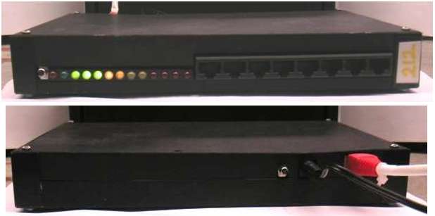
Example: The A2037E gets its power from a power adaptor that you plug into an AC wall socket. It communicates with the outside world via TCPIP over Ethernet. There is an RJ-45 socket on the back side of the driver for 10-Base-T Ethernet. On the front side are eight RJ-45 sockets for root cables. The sockets are numbered one through eight, with number one next to the indicator LEDs and number eight farthest from the LEDs.
Example: The LWDAQ Driver with VME Interface (A2037A) is a 6U VME board for use in large LWDAQ systems. The A2037A provides eight driver sockets and occupies 512 KBytes of address space.

A LWDAQ Server is the combination of a TCPIP connection and one or more LWDAQ Drivers. The portion of a LWDAQ Server that receives and interprets TCPIP messages is a LWDAQ Relay. Each server has only one relay.
Example: We use the A2037A in conjunction with the VME-TCPIP Interface (A2064). The A2064 provides communication with all drivers in its VME crate through a single Ethernet connection. We select a driver socket by specifying the driver's base address and the socket number. In the figure above, each VME crate is a LWDAQ Server. Each crate contains a single TCPIP-VME Interface (A2064F) and twenty LWDAQ Drivers (A2037A). Each server provides 160 driver sockets. Each driver socket connects to a multiplexer at the end of roughly 100 m of root cable. Each multiplexer is connected to an average of eight devices. Each of these servers therefore provides access to roughly one thousand devices.
A LWDAQ Server accepts TCPIP connections to its IP address on a user-configurable port number. It responds to TCPIP messages that conform to the LWDAQ Message Protocol or the SIAP Message Protocol. We describe both protocols in TCPIP Messages. The server decides on start-up to use the SIAP protocol if its server port number lies in the range 30,000 to 40,000. Otherwise it will use the LWDAQ protocol.
Example: The LWDAQ Driver with Ethernet Interface (A2037E) uses an RCM2200 TCPIP Module to implement its LWDAQ Relay. The VME-TCPIP Interface (A2064A) does the same. The faster VME-TCPIP Interface (A2064F) uses an RCM3200.
The part of a LWDAQ Server that transmits and receives electrical signals to and from LWDAQ Devices is called a LWDAQ Controller. A single server can contain many LWDAQ Controllers.
Example: The LWDAQ Drivers with Ethernet Interface A2037E and A2071E are self-contained LWDAQ Servers with a single LWDAQ Relay and a single LWDAQ Controller and eight driver sockets. The VME crate LWDAQ Servers shown in the figure above each contain a single LWDAQ Relay and twenty LWDAQ Controllers.
The Configurator Tool and the Diagnostic Instrument both allow you to determine the hardware identifier and hardware version of both the relay and the controller in a LWDAQ Driver. The identifier tells us the type of relay or controller. The version keeps track of modifications to the deisn.
| Assembly | Identifier | Description |
|---|---|---|
| A2037A | 37 | controller with VME interface |
| A2037E | 37 | relay and controller |
| A2064A | 64 | relay with VME interface, RCM2200 TCPIP server |
| A2064F | 64 | relay with VME interface, RCM3200 TCPIP server |
| A2087A | 87 | relay with VME interface, RCM6700 TCPIP server |
| A3038C | 38 | integrated relay, controller and device, RCM6700 TCPIP server |
We connect to a LWDAQ Server with a LWDAQ Client. The client runs on a computer somewhere on the same TCPIP network as the server. Our client software runs on Windows, MacOS, and Linux. We describe our LWDAQ Software in the next section.
It is possible for you to write your own software to send and receive messages to and from the LWDAQ over TCPIP. We know of at least one lab that has a direct interface from LabView to LWDAQ using the LWDAQ Message Protocol. Nevertheless, we have done our best to provide you with a program that communicates with the LWDAQ hardware, acquires data, and analyzes the data. Our LWDAQ Software is a combination of analysis routines written in Pascal and communication and graphics routines written in TclTk.
The foundation of our LWDAQ Software is a TclTk interpreter. The interpreter executes TclTk scripts that communicate with the LWDAQ hardware over TCPIP. It generates the graphical user interface. It loads our analysis library and makes its routines available to our scripts as TclTk commands. You will find all the TclTk scripts that define LWDAQ and its instruments in Sources. The first script that LWDAQ runs is Init.tcl.
We perform computationally-intensive data analysis with routines defined in the Pascal programming language. The source code is easy to read, well-commented, and acts as a reference for the analysis functions. Starting with LWDAQ 10, we compile our Pascal code with the open-source Free Pascal Compiler and produce 64-bit binaries for Linux, Windows, and MacOS. (In earlier versions of LWDAQ, we used the open-source GNU Pascal Compiler to generate 32-bit binaries all three platforms, and added 64-bit binaries for Linux in LWDAQ 8.) We compile the analysis routines into a shared libraries called lwdaq.so_Linux, lwdaq.so_Windows, or lwdaq.so_MacOS. If you want to use our analysis routines with your own application, follow the instructions in Rasnik Manual for compiling liblwdaq, a dynamic library to which you can link your application.
The TclTk interpreter is an open source application. TclTk is a scripting language understood by TclTk interpreter programs, in the same way that UNIX is a scripting language understood by a UNIX shell. As a TclTk reference manual, we recommend Practical Programming in TclTk. The TclTk interpreter, called the Wish Shell, exists for almost every computer operating system. The Wish Shell is bundled with MacOS, and usually installed with Linux. You can download it yourself for Windows. Once you install and run the interpreter on your computer, and it will run any TclTk script. The following script opens a socket to IP address lwdaq.hep.brandeis.edu port 90, and then closes the socket.
set sock [socket lwdaq.hep.brandeis.edu 90]
close $sock
It does not matter what platform you are on, the same script works because all the platform-dependence of opening and using a TCPIP socket has been taken care of and hidden from you by the TclTk interpreter. The following script creates a button that writes Hello World to the console every time you click on the button with the mouse.
button .helloworld -text "Hello World" -command "puts {Hello World}"
When you start our LWDAQ program, you start a TclTk interpreter (a Wish Shell). We have changed its appearance, but it is still a Wish Shell. You will come across the name Wish and the TclTk feather icon in odd places as you use the program. When the LWDAQ program starts up, it runs our initialization scripts, loads the analysis library, and creates our LWDAQ user interface. The File, Instrument and Tool menus appear in the LWDAQ menu bar. The Instrument menu opens windows that control the various LWDAQ instruments. Each instrument performs a particular type of data acquisition and analysis.
Example: The BCAM Instrument acquires images from BCAM devices.
The windows opened by the Instrument Menu are the instrument panels. Each instrument panel allows you to control one of the instruments. We can control the instruments from the command line also, without using the panels. The non-graphical version of LWDAQ runs with only a terminal interface, and the no-console version runs in the background without even a terminal.
If you have your own Driver with Ethernet Interface (A2037E), connect it to your laptop directly with a cross-over Ethernet cable and configure its TCPIP interface to suit your local area network with the help of the Configurator tool in the Tool menu. Once you have your devices connected to your driver, and the driver connected to the Internet, you can display and record measurements from your LWDAQ Devices (hardware objects) using the LWDAQ Instruments (software routines).
You may want to use several instruments in an experiment. You may want record measurements to disk and take data in a continuous cycle. You can combine instruments and record data with our Acquisifier Tool. You can create your own tool to define your own window with buttons and a display. You create a tool by defining it with a TclTk script. You can run your tool from the Tool Menu, or you can put the tool in the Configuration directory and have LWDAQ run the tool automatically at start-up. We describe how to create tools in the Tools section.
Example: The Spectrometer Tool uses the RFPM Instrument to plot a graph of power density versus frequency. The BCAM Calculator calls no instruments, but analyzes calibration data on disk. The BCAM Calibrator obtains BCAM calibration data.
In your scripts, you can call the LWDAQ Script Commands, the names of which all start with the letters LWDAQ, and our LWDAQ Library Commands the names of which all start with the letters lwdaq. The script commands are defined by the TclTk scripts executed by the LWDAQ program at start-up, or when you select Re-Initialize from the File menu. The library commands are contained in a shared library called lwdaq.so that we pre-compile for you from our Pascal source code. The LWDAQ program loads the LWDAQ dynamic library at start-up, and calls its initialization routine. The initialization routine installs the lwdaq commands in the TclTk interpreter. These commands are now available in the console, and for use in TclTk scripts. We describe our LWDAQ procedures in the Commands and list them individually in the LWDAQ Command Reference.
When the LWDAQ program connects to a LWDAQ Driver, it does so over TCPIP. All our instruments and tools use the LWDAQ_socket_open routine declared in the Driver.tcl script file to open the TCPIP connection to a driver. To open a TCPIP socket, we must specify an IP address and a port number. The LWDAQ_socket_open routine will accept either a numerical address or a host name. You specify the port number by adding it to the end of the IP address, separated from the address itself by a colon, like so:
LWDAQ_socket_open lwdaq.hep.brandeis.edu:90
By default, we use port number 90 on the LWDAQ Driver with Ethernet Interface (A2037E) and the VME-TCPIP Interface (A2064). If you do not specify a port number, LWDAQ assumes you are trying to connect to port 90. The LWDAQ's TCPIP can be re-programmed, however, to accept connections on different port number.
You specify the driver socket you want to use to communicate with your target device using the LWDAQ_set_driver_mux routine. Sometimes there is more than one LWDAQ Driver associated with the TCPIP socket you have opened. For example, if you have a VME-TCPIP Interface (A2064) plugged into a VME crate, you might have twenty LWDAQ Driver with VME Interface (A2037A) in the crate, and to select one of them you need to specify its base address to the VME-TCPIP interface. The LWDAQ software combines the act of selecting a drivers socket with the act of selecting a driver. You specify the base address of the driver with an eight-digit hex number.
LWDAQ_set_driver_mux $sock 00E00000:1 3
The above command selects the driver at base address hexadecimal "00E00000". It selects socket 1 on that driver, and transmits an address word down this socket to direct a multiplexer, if there is one connected, to select branch socket 3. We can specify the base address in a more abbreviated way, so long as the base address begins with two zeros and ends with four zeros.
LWDAQ_set_driver_mux $sock E0:1 3
The above "E0" is equivalent to "00E00000". In the following command, we have left out the base address, and select driver socket 1 and branch socket 3.
LWDAQ_set_driver_mux $sock 1 3
The The LWDAQ program stores all its measurements as two-dimensional arrays of bytes, which we call images. The measurement received from a camera really is an image, and we have found that the same format will accomodate any instrument we care to invent. All images are maintained by the compiled Pascal procedures. Here's the TclTk script command that draws an image with name an_image in a TK photo (drawing area in a window) with name a_tk_photo:
lwdaq_draw an_image a_tk_photo
If you want to intensify the image and zoom it, you can do so like this:
lwdaq_draw an_image a_tk_photo -intensify exact -zoom 2
We illustrate the LWDAQ image drawing and graph plotting in our Boltzmann Simulation script. Download it, open it with the Load button in the Toolmaker (the Toolmaker is in the Tool menu). Press Execute and you will see two graphs on the screen, one of which is evolving to look like the other. If you inspect the code, you will see how the plotting and drawing is done.
Look at the Intensification section below for a description of the intensification options. Open the Camera instrument, press Read, navigate to the LWDAQ/Images directory and choose an image to display. Now open the console using the File menu. Type the following and press return:
LWDAQ_acquire Camera
You will see the Camera capture a new image. The console will show the result returned by your TclTk command. The result is a the name of the image you captured and a string of numbers giving characteristics of the image. You can do the same for any of the instruments defined in the Instrument menu, and each of them will return a string with an image name and results. The data acquisition will take place whether the instrument panel is open or not. To understand what the results are, look at the section in this manual that describes the instrument, or set verbose_result to 1 in the instrument panel, and acquire again.
We call custom scripts tools. Tools are simply text files containing TclTk commands that you can execute from LWDAQ. We provide a number of them in the Tool Menu, written by ourselves and other LWDAQ users. You can write your own to manage your own data acquisition system, and run them on any computer upon which you have installed the LWDAQ software. If your desktop computer runs Windows, but your lap-top runs MacOS, you will use the same tool on both computers. The LWDAQ is not tied to any computer or any operating system. You can access your data acquisition system from anywhere in the world, or you can keep it private on a local area network.
As an introduction to programming using LWDAQ commands, we invite you to take a look at our Boltzmann Simulation demonstration script. This script does no data acquisition, but it illustrates how you can develop plotting and calculating tools with the help of the LWDAQ Toolmaker. Or you could try looking at our sudoku-solving tool. You will find the Sudoku tool in the Tools/More menu, and you will find its script in the Tools/More directory.
There are two ways to install LWDAQ. The first way is to clone our github repository. The advantage of installing LWDAQ with the git utility is that you can update your installation easily using a couple of git commands. In a Terminal, enter the following command to intall LWDAQ.
git clone https://github.com/OSI-INC/LWDAQ
You will now have the very latest version of LWDAQ. To go to an earlier, stable version, you can use the git checkout command, like this:
git checkout v10.5.5
If we fix a bug in the code for you, you can update your distribution with:
git stash
git pull
The pull command updates all files, but leaves your core, instrument, and tool settings intact. The only disadvantage of the git installation presents itself on MacOS, where the git repository does not provide a pre-installed LWDAQ graphic for the LWDAQ icon.
The second way to download and decompress the LWDAQ zip archive. You will find the latest version of our software at our Software page. The ZIP same archive works on all platforms. Download and extract the LWDAQ directory. Avoid placing LWDAQ directory in a directory tree that has spaces in its directory names. If you see other directories and files in the zip archive, ignore them: they belong to another operating system. In the LWDAQ directory structure, you may see files with names beginning with a period. These you can ignore or delete. They are artifacts of another operating system. The archives contain three versions of the TclTk interpreter, one each for Linux, Windows, and MacOS.
The following subsections discuss further details of installation particular to each of our supported operating systems: Linux, MacOS, Raspbian and Windows.
[02-OCT-23] In a Linux terminal, go to the LWDAQ directory and start LWDAQ with the following command.
./lwdaq
The LWDAQ process will open a small window with a Quit button and the LWDAQ menus. The terminal will be taken over by LWDAQ as well, acting as a console for the LWDAQ command interpreter. If you want to launch LWDAQ as a separate process with graphics, and continue using your terminal, use the following command.
./lwdaq --spawn
When you run LWDAQ like this on Linux, there is no LWDAQ command interpreter available. The lack of a command interpreter is unlikely to cause you any inconvenience until you decide to start writing LWDAQ scripts of your own. But at that time, you can use the Toolmaker to execute commands and see their results. In the long run, we plan to add a Slave Console to the Linux version of LWDAQ, just as there exists in the File menu of the MacOS and Windows versions of LWDAQ.
To exercise LWDAQ, open the Camera instrument from the Instrument menu. Press Read and select an image from LWDAQ/Images to display. Everything you need to run LWDAQ is contained in the LWDAQ application bundle. The other files and directories contain example Tools, of which the Configurator is the one you are most likely to need, example images, and the Pascal source code. The lwdaq command calls the TclTk or Tcl interpreter included with our LWDAQ distribution. By default, the command launches the graphical version of LWDAQ. See Run from Terminal for options to launch LWDAQ without graphics, in the background, and as a participant in a piped process.
To create a desktop icon for LWDAQ on Ubuntu Linux, navigate to the LWDAQ directory with a Terminal and enter the following command.
./lwdaq LWDAQ.app/Contents/Linux/desktop-file-create.tcl
sudo desktop-file-install ~/Desktop/lwdaq.desktop
Right-click on the lwdaq.desktop and select "Allow Launching". The desktop file should now show the LWDAQ graphic. Double-click on the icon and LWDAQ will launch. The graphical user interface will start up and a dedicated terminal will open up as well, acting as the LWDAQ command interpreter.
We build our Pascal analysis library on Linux from the terminal with a Pascal compiler and GNU Make. Our LWDAQ distribution comes with pre-compiled libraries, but if you want to modify our Pascal source code and re-compile, install the Free Pascal Compiler via the FPC download page. Go to the LWDAQ/Build directory and type make. The make procedure will build lwdaq.so_Linux and install it in the correct place in the LWDAQ directory tree.
To provide the TclTk interpreter upon which the LWDAQ software is built, we download the source code from Source Forge and compile on Debian Linux. We download the TclTk sources. Starting with LWDAQ 10.1, LWDAQ uses TclTk 8.6 on Linux. To build Tcl, we move to the tcl/unix directory in the source distribution and enter the following command.
./configure --prefix ~/build --exec-prefix ~/build
make
make install
In the configure step, we must specify an absolute path for the prefix directories, but the tilda for home will work. When the configure, make, and install are done, we check that the Tcl binaries and libraries are installed in our build directory. We go through the same procedure in the tk/unix directory, with the same three command lines. When the Tk configure, build, and install are complete, we move the ~/build/lib and ~/build/bin folders into LWDAQ.app/Contents/Linux and our TclTk for Linux LWDAQ is complete.
[02-OCT-23] Having downloaded and decompressed the LWDAQ zip archive, move the LWDAQ application out of the LWDAQ folder and onto your desktop. Move it back into the LWDAQ folder. This deliberate removal and replacement tells the operating system that you know of and accept the existence of the application. Now you can run LWDAQ without the security precaution known as translocation. Double-click on the LWDAQ icon. The operating system tells us that it will not run LWDAQ. Open System Preferences and select "Security & Privacy", and select the "General" tab. Check the box that says you really want to run LWDAQ. Now double-click on the LWDAQ icon again, and select "Open" instead of the default "Cancel". You should see the LWDAQ main window open. It has only one button in it, which says "Quit".
The LWDAQ icon is a folder called LWDAQ.app. The extension .app is usually hidden by the Finder, depending upon how you have your Finder configured. You can see what is inside the LWDAQ.app directory by control-clicking on the LWDAQ.app icon and selecting Show Package Contents. We can launch LWDAQ by double-clicking on the icon, or we can open a terminal, navigate to the LWDAQ directory and enter:
./lwdaq
The LWDAQ window with the Quit button will appear. Your terminal will be taken over by LWDAQ to act as a command interpreter. By default, the command launches the graphical version of LWDAQ. See Run from Terminal for options to launch LWDAQ without graphics, in the background, and as a participant in a piped process. You can run LWDAQ as a process independent of your terminal with --spawn option.
./lwdaq --spawn
When launched with the --spawn option, LWDAQ provides a dedicated slave console that you can open with Show Console in the File menu. The original terminal from which you launched LWDAQ will be freed for your continued use. The slave console runs in a separate window accompanied by its own menus. To get back to the original LWDAQ menus, click on one of the LWDAQ windows.
To exercise LWDAQ, open the Camera instrument from the Instrument menu and press Read. Select an image from the LWDAQ/Images folder to display. Everything you need to run LWDAQ is contained in the LWDAQ application bundle. The other files and directories contain example Tools, of which the Configurator is the one you are most likely to need, example images, and the Pascal source code.
Our LWDAQ distribution comes with pre-compiled libraries for MacOS. If you want to re-compile the analysis libraries for yourself, you need to install a Pascal compiler and GNU Make. You may have make available at the command line on your MacOS machine, you may not. If not, install it with Command Line Tools, or with Home Brew. Now install the Free Pascal Compiler. Do not install FPCB with Home Brew; go directly to the FPC download page and get the 64-bit MacOS version. Having installed FPC, go to the LWDAQ/Build directory and type make. The make will build lwdaq.so_MacOS and install it in the correct place in the LWDAQ directory tree.
We build our Tcl and Tk interpreters from sources, which we obtain from the Tcl Developer Exchange. The source distribution contains two directories named tclx.y.z and tkx.y.z, which we rename tcl and tk. Starting with LWDAQ 10.2, LWDAQ uses TclTk version 8.7 on MacOS. To build the TclTk application we need the MacOS command line tools. Type "cc --version" in the terminal. If you get the CLANG compiler version, you can proceed with the build. Otherwise, MacOS will guide you through installation of the command line tools. Once you have these installed, use the following commands in the directory containing both the tcl and tk directories.
export CFLAGS="-arch x86_64 -mmacosx-version-min=10.9"
make -C tcl/macosx embedded
make -C tk/macosx embedded
We specify x86_64 to make sure we produce a 64-bit binary for Intel processors. We specify the minimum MacOSX version 10.9 so that LWDAQ will run on MacOS 10.9 or later. These commands create a build directory. In build/tcl is a file called tclsh8.7. This is the console-driven, non-graphical Tcl shell program, which we use for the no-gui version of LWDAQ on MacOS. We re-name the file tclsh. We make the shell reference to its own libraries relative to its own location with the install_name_tool as follows.
install_name_tool -change \
  /Library/Frameworks/Tcl.framework/Versions/8.7/Tcl \
  @executable_path/../Frameworks/Tcl.framework/Versions/8.7/Tcl \
  tclsh
You can check that you have done this right with the otool utility.
otool -L tclsh
In build/tk is an application bundle called Wish.app. This is the TclTk shell program, or wish shell (windowing shell). We use this application bundle as starting-point for our LWDAQ directory structure. We rename it LWDAQ.app. We place our tclsh executable in the LWDAQ.app/Contents/MacOS directory alongside the Wish executable. The following commands tell you which platforms your particular executables will work on.
lipo -info LWDAQ.app/Contents/MacOS/Wish
lipo -info LWDAQ.app/Contents/MacOS/tclsh
[05-MAR-23] The Raspbian operating system is GNU Linux compiled for the Broadcom ARM processor. There are 32-bit and 64-bit versions. We do not provide TclTk interpreters embedded in LWDAQ for Raspbian. You must install TclTk on the Raspberry Pi yourself. Starting with LWDAQ 10.4.3, however, we provide a compiled 32-bit version of our analysis library, which we call lwdaq.so_Raspbian. This library runs on 32-bit Raspbian. We tested the library on Stretch and Bullseye. The Pascal compiler still has some problems on Raspbian: when we compile and run our test program, it crashes in a particular place. But most analysis routines will work, such as those that render images. To install, download and expand the LWDAQ zip archive, navigate to the LWDAQ directory and try the following.
sudo apt update
sudo apt upgrade
sudo apt install tclsh
sudo apt install wish
./lwdaq
If the graphical LWDAQ opens up with no errors, you are all set. Assuming LWDAQ starts up without errors, running LWDAQ on Raspbian is identical to running it on Linux. If, however, you see libarary load errors, you must compile our analysis library for your platform and link it to your own TclTk, which our Makefile will do for you. Navigate to the LWDAQ/Build directory and enter the following commands.
sudo apt install fpc
make
cd ..
./lwdaq
These commands install the Free Pascal Compiler, build our library, and launch LWDAQ. The make compiles our LWDAQ analysis library. We find this re-compile works on Stretch Raspbian, but not Bullseye. We are still trying to figure out why we cannot compile a working library on Bullseye.
[02-OCT-23] Download the LWDAQ zip archive and extract the LWDAQ directory to a location of your choice. Do not extract any other directories: they are artifacts of another operating system. Attempt to start LWDAQ by double-clicking on the LWDAQ.bat file. The first time you try to run LWDAQ, several barriers will be put up to stop you. Anti-virus software will try to quarantine the lwdaq.so_Windows dynamic library, declaring that it contains routines that are capable of damaging your operating system. We suggest you right-click LWDAQ.bat, select Properties, under the General tab, select "Unblock", and apply changes. If that fails, you must somehow direct the anti-virus software to restore the library to its original location. After that, Windows will ask if you are really sure you want to run LWDAQ. Be firm and resolute with the operating system and it will eventually yield to your will and run our program. You should see the LWDAQ main window open up.
If you would like LWDAQ icon on your desktop, to make it easier to open the program in the future, make a shortcut to the LWDAQ.bat file. Place the shortcut on your desktop. Right-click on the shortcut file and select Properties. Click Change Icon and browse for the lwdaq.ico file in your LWDAQ\LWDAQ.app\Windows folder. Click OK twice. Your shortcut will now have the LWDAQ icon, and LWDAQ will open when you double-click on the icon. Another way to run LWDAQ is from the DOS command line. Open a DOS command shell, navigate to the LWDAQ directory and enter:
LWDAQ.bat
The LWDAQ program will start up with graphics. The command shell will show some start-up information from running the batch file, but otherwise will be available to you for further commands, or you can close it. To run LWDAQ without graphics, use the --no-gui option. The LWDAQ process will take over the command shell to act as its standard input and output.
LWDAQ.bat --no-gui
We can also run LWDAQ within one of the Linux emulators available on Windows. The lwdaq file is a Bash script. You can run it on Windows only within a Linux emulator. Our favorite Linux emulator is the Git-Bash shell that comes with Git for Windows. If you use Git-Bash you can clone our LWDAQ repository and pull the latest version when we make modifications, or revert to earlier versions if you have a problem with an update. Alternatively, follow these instructions to configure the built-in Linux shell, or download and install a third-party Linux emulator such as MSYS. All emulators give you a linux Bash Shell in which you can run the lwdaq program, as we describe in Run From Terminal.
The DOS shell does not recognize lwdaq as an executable. When you enter lwdaq in the DOS shell, the shell looks for a file called lwdaq.bat. But DOS is case-insensitive, so it accepts LWDAQ.bat as a match, and runs it. Thus we see that the same lwdaq command works on Windows as well as Linux-like platforms, so that the same lwdaq terminal command can be used to launch LWDAQ on any platform.
Our LWDAQ distribution comes with pre-compiled analysis libraries for Windows. But if you want to edit our Pascal source code and re-compile for yourself, you will need a Pascal compiler. We build our Pascal analysis library on Windows with a pascal compiler and GNU Make running in a Unix emmulator. To replicate our build procedure, install MinGW, which includes a Linux shell and GNU Make. Go to the MinGW Download Page. Download and run the Automated MinGW Installer. Install the bare minimum files of MinGW. Go back to the same download page and download the most recent version of the MSYS shell program for MinGW. We end up with an icon on your desktop for the MSYS shell. When we double-click on the icon, a Unix terminal opens up. Install the Free Pascal Compiler, or FPC. At the time of writing, the FPC compiler for Windows is a 32-bit executable that will compile for 64-bit. Having installed FPC, go to the LWDAQ/Build directory and type make. The make procedure will build lwdaq.so_Windows and install it in the correct place in the LWDAQ directory tree.
The TclTk interpreter we bundle with LWDAQ for Windows is a binary we downloaded from the repository provided by Thomas Perschak. Starting in LWDAQ 10.1, we use TclTk 8.6 on all Windows platforms. You will find the wish and tcl shells, and the Tcl and Tk libraries in the LWDAQ.app/Contents/Windows directory.
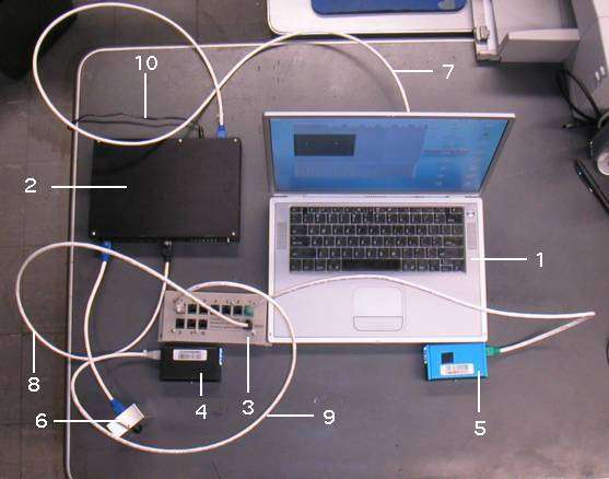
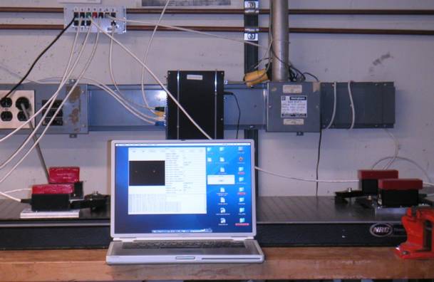
The figure below shows an example LWDAQ system. The lap-top is connected to the local wireless network. The driver is the black box on the wall. It is connected to the local wired network. The lap-top acquires data from the devices connected to this driver. It can acquire data from devices connected to other drivers as well.
Here are instructions for setting up your LWDAQ Hardware. Note that these instructions apply both to systems that use a LWDAQ Driver with Ethernet Interface, such as the A2037E and to systems that use a TCPIP-VME Interface, such as the A2064. In the latter case, the LWDAQ Drivers with VME Interfaces, such as the A2037A, will reside in a VME crate along with the TCPIP-VME Interface, and when considered as a whole, the VME crate is equivalent to a single LWDAQ Driver with Ethernet Interface, only with many more driver sockets.
If you make it through these steps, you are now ready to open the instrument that applies to your LWDAQ Device. If it's a BCAM, go to the BCAM Instrument section of this manual for instructions on how to use the device.
Here is the directory tree of our LWDAQ software distribution archives. Each archive contains all the files and directories needed for all supported platforms.
lwdaq     {Call from terminal to start LWDAQ}
LWDAQ.bat {Double-click to start LWDAQ on Windows}
LWDAQ.app {Double-click to start LWDAQ on MacOS X}
  Contents
    LWDAQ
      Info.plist {MacOS}
      PkgInfo {MacOS}
      Resources
        Scripts
          AppMain.tcl {MacOS launch script}
        LWDAQ.sdef {MacOS}
        LWDAQ.icns {MacOS}
        LWDAQ.gif {Generic}
      MacOS
        {MacOS TclTk interpreter}
        {MacOS Tcl interpreter}
      Frameworks
        {MacOS TclTk libraries}
      Windows
        {Windows TclTk interpreter}
        {Windows Tcl interpreter}
        {Windows TclTk libraries}
        {Windows icon}
      Linux
        {Linux TclTk interpreter}
        {Linux Tcl interpreter}
        {Linus TclTk libraries}
        {Linux icon}
        {Linux Desktop File}
      LWDAQ
        License.txt
        CRT.html {command reference template HTML file}
        Init.tcl {initializes global arrays and calls other scripts}
        Utils.tcl {utility routines}
        Driver.tcl {tcpip communication with driver}
        Interface.tcl {graphical user interface}
        Instruments.tcl {instrument management routines}
        Tools.tcl {tool routines}
        Toolmaker.txt {saved toolmaker scripts}
        Instruments
          BCAM.tcl
          Camera.tcl
          Diagnostic.tcl
          Dosimeter.tcl
          Flowmeter.tcl
          Gauge.tcl
          Inclinometer.tcl
          Rasnik.tcl
          Receiver.tcl
          RFPM.tcl
          SCAM.tcl
          Terminal.tcl
          Thermometer.tcl
          Viewer.tcl
          Voltmeter.tcl
          WPS.tcl
        Configuration
          {settings files}
        Modes
          {operational mode scripts}
        Packages
          {tcl-compatible packages for dynamic loading}
        Temporary
          {temporary scripts used for spawning}
        lwdaq.so_MacOS {Macos Intel 64-bit analysis library}
        lwdaq.so_Linux {Linux 64-bit analysis library}
        lwdaq.so_Windows {Windows 64-bit analysis library}
        lwdaq.so_Raspbian {Raspberry Pi 32-bit analysis library}
Tools
  Acquisifier.tcl
  Analyzer.tcl
  BCAM_Calculator.tcl
  BCAM_Calibrator.tcl
  Configurator.tcl
  CPMS_Calibrator.tcl
  CPMS_Manager.tcl
  Fiber_Positioner.tcl
  Image_Browser.tcl
  Saturator.tcl
  Spectrometer.tcl
  Startup_Manager.tcl
  Stimulator.tcl
  Wire_Monitor.tcl
  More
    {more tools}
  Spawn
    Neuroplayer.tcl
    Neurorecorder.tcl
    Videoarchiver.tcl
  Data
    {data files for tools}
Sources
  {Pascal sources for lwdaq analysis library}
  {TclTk sources for LWDAQ Platform}
  {TclTk sources for LWDAQ Instruments}
Images
  {sample images}
Build
    Makefile {compile from terminal on all platforms}
    p.pas {example pascal program}
    test.pas {test routines for analysis library}
    archive {archiving utility we use to upload new releases}
license.txt {GNU Public License}
readmen.md {Readme file in markdown format}
On MacOS, the Finder by default hides the .app extension of LWDAQ.app. Instead of a file called LWDAQ.app, the Finder shows you an icon called LWDAQ. Double-click on the icon, and LWDAQ opens up. On Windows, the file Explorer hides the .bat extension, but will show you the LWDAQ.app file name in full. Double-click on the LWDAQ file.
The main window has a quit button. You can quit the program by pressing the quit button, closing the main window, selecting Quit from the LWDAQ menu, or pressing apple-q on MacOS and control-q on Linux. The LWDAQ main window has the following menus on all platforms: LWDAQ, File, Tool, Instrument.
LWDAQ_open Diagnostic
The Tool/Edit menu provides Run Tool, Edit Script, New Script and Toolmaker commands. The Run Tool command opens a file and executes it as a TclTk script. The script will execute at the TclTk global scope. It will have access to all LWDAQ commands. The Edit Script command opens an existing script file in a text editor, while New Script starts the creation of a new file. The Toolmaker command opens the Toolmaker, which combines a text editor with script execution and a history of executed scripts. The TclTk console that comes with the Linux version of LWDAQ does not have a command history, so the Toolmaker is particularly useful on Linux for testing data acquisition scripts.
The Tool/Spawn menu lists tools that will be launched as processes that run independently of the main LWDAQ program. When we spawn a tool, we create a new LWDAQ process that provides only the tool functionality. The new LWDAQ process runs independently of the original LWDAQ process. The spawned processes will continue to run even after the original LWDAQ process crashes or quits. Because spawned tools are independent, they will collide with one another when acquiring data from the same LWDAQ system. Most collision will be resolved by waiting a short time, but some collisions cannot be resolved without disruption of measurements or loss of data.
The Tool/Run menu lists tools that will run within the main LWDAQ process. These tools will close when we quit the LWDAQ main program, and they will turns using the LWDAQ Instruments when acquiring data. None of them will collide or conflict with one another when acquiring data from the same LWDAQ system. The Run Submenu contains an entry for each tool LWDAQ finds in the Tools directory at start-up. Select the tool and its window will open.
The linear dimensions of all images presented by LWDAQ instruments are controlled by the value of the global display_zoom parameter. By default, this parameter is one. On most platforms, display_zoom = 1.0 produces images of a satisfactory default size. But on some monitors, the images are too small, and on rare low-resolution monitors, the images are too large. We can enlarge all images by setting display_zoom to an integer value greater than one. We can reduce images by setting display_zoom to an integer fraction, such as 0.5, 0.33, or 0.25.
The display_zoom parameter is available in the Library Settings panel of the System Monitor. To change display_zoom temporarily, we enter a new value in the Library Settings panel and press Apply. To make this change permanent, we select Save Settings from the File Menu. The next time we open LWDAQ, our saved value of display_zoom will be recalled.
In addition to the global display_zoom, each instrument has its own zoom parameter that we can apply on top of the global display_zoom. The instrument zoom parameter is available in its Info Panel. We can save the settings of an instrument with the Save Settings button in the Info panel.
Global display settings gamma_correction, rggb_blue_scale, and rggb_red_scale affect the hue of color images. Printing of numerical results by library routines are affected by fsr (field size real), and fsd (field size decimal). We describe these and all other global library options in our lwdaq_config manual entry. All these parameters may be adjusted and saved with the Library Settings panel and the Save Settings command.
[02-FEB-24] The Configurator allows you to communicate with a LWDAQ Server, read its configuration parameters from RAM, and write new configuration parameters to EEPROM. Examples of LWDAQ Server are the LWDAQ Driver with Ethernet Interface (A2071E), VME to TCPIP Interface (A2087), and the Animal Location Tracker (A3038). The Configurator is a LWDAQ Tool defined by the Configurator.tcl script in the Tools directory. Select Configurator from the Tool menu. The Configurator Window will appear.
Example: The LWDAQ Driver with Ethernet Interface (A2037E) provides a LWDAQ system with eight driver sockets and one TCPIP interface. The A2037E is a self-contained LWDAQ Server, with both the LWDAQ Relay and LWDAQ Controller in the same enclosure. The Configurator tries to contact the A2037E with contact_ip_addr and contact_ip_port.
Example: A VME crate contains twenty LWDAQ Drivers (A2037A) and a single TCPIP-VME Interface (A2064) provides a LWDAQ Server with 160 driver sockets. Each A2037A provides a LWDAQ Controller. The A2064 provides a LWDAQ Relay that provides TCPIP communication for all twenty controllers. The Configurator contacts the A2064 using contact_ip_addr and contact_ip_port. It identifies an individual A2037A in the crate with contact_base_addr.
The contact_base_addr parameter contains the thirty-two bit hexadecimal base address of an individual driver in a LWDAQ. When contact_base_addr is 00000000, the Configurator assumes a LWDAQ Server with only one LWDAQ Controller. With a non-zero base address, the Configurator assumes a LWDAQ Server with one LWDAQ Relay but multiple LWDAQ Controllers, each of which you select with a unique base address. The Configurator reads out a variety of identifiers and version numbers. These allow you to confirm the kind of hardware the Configurator is talking too, as shown in the Identifier Table above.
The first step in the Configuration process is to make contact with your LWDAQ Relay over TCPIP. If you are trying to communicate with an Animal Location Tracker (ALT) or Telemetry Control Box (TCB), you get the IP address of its LWDAQ Relay by looking at the last three digits of its serial number. Serial number S0103 is ip address 10.0.0.103 and number P71038 is 10.0.0.38. If you are trying to communicate with a LWDAQ Driver (A2071E) that is fresh from the factory, it's IP address will be 10.0.0.37. Apply power to the relay and connect it directly to a computer. The computer and the relay now form an isolated two-node Internet. What you must do next is configure your wired ethernet interface to operate on subnet 10.0.0.x. You assign your own computer IP address 10.0.0.2 on the wired ethernet interface, and set the wired interface's "subnet mask" to 255.255.255.0. You leave the "gatway" of your ethernet interface blank, so as to make sure the computer never tries to use your wired network to communicate with the outside world.
On MacOS, create a new location with the Locations Manager, which is accessible through the Networks icon in System Settings. Select your wired Ethernet connection and configure it using the graphical user interface of the Locations Manager. We have specific instructions for Windows 7 and Windows 10. On all Windows platforms, disable "NetBIOS over TCP/IP". On Linux, you edit file /etc/dhcpcd.conf to configure your wired ethernet interface, which may be called eth0, or may be called something rediculously cryptic if you have "predictable interface names" on your version of Linux.
Now that your computer and the relay are connected together, and, we assume, operating on the 10.0.0.x subnet, enter 10.0.0.37 in the contact_ip_addr box in the Configurator. Make sure that contact_password, contact_ip_port, and contact_base_addr are LWDAQ, 90, and 00000000 respectively. Press the Contact button. The Configurator will tell you whether it can contact the driver. If it makes contact, it will report the relay's MAC address and version numbers.
Attempting to open socket...success.
Attempting login...success.
Relay Software Version: 12
Relay MAC Address: 0090c2c1905f
Controller Hardware ID: 37
Controller Hardware Version: 1
Controller Firmware Version: 11
Closing socket...closed.
If the Configurator cannot make contact with your LWDAQ Relay, try resetting the LWDAQ's EEPROM configuration file with the following procedure. Find the Configuration Switch on your relay. This button is next to the shielded Ethernet jack on the A2037E. It is on the top side of the board on the A2064 and A2101. Press and hold the Configuration Switch. Now press the Reset Switch while still holding down the Configuration Switch. The Reset Switch is on the front side of the A2037E next to the indicator LEDs, on the front panel of the A2064, and on the top side of the A2101. Release the Reset Switch. Keep holding the Configuration Switch for at least three seconds. The relay re-boots. It notices that the Configuration Switch is pressed. It re-writes its configuration file, which is stored in its non-volatile (EEPROM) memory. It loads the newly-written values into RAM and starts its server socket. In case our written descriptionis unclear, we have an additional LWDAQ Driver Reset video that may clarify the details and timing of the procedure.
ip_addr: 10.0.0.37
gateway_addr: 10.0.0.1
subnet_mask: 255.255.255.0
ip_port: 90
password: LWDAQ
operator: relay_version_15
security_level: 1
tcp_timeout: 0
configuration_time: 00000000000000
driver_id: none_assigned
Configuration parameters must not contain any white-space characters, colons (:), semi-colons (;), or commas (,). They may contain periods (.) and dashes (-) and underscores (_).
Try again to contact the LWDAQ Relay with the Configurator's Contact button. If you don't succeed, check your cables. Look at the lights on the relay. The two yellow lights nearest to the Reset Switch on an A2037E or A2064A/F are Link and Activity indicators. One should be on permanently when your cable is plugged into the shielded Ethernet socket. Don't be distracted by the eight unshielded RJ-45 sockets on the front of the A2037E. These are not Ethernet sockets. They are the LWDAQ Driver Sockets. If you don't get a Link light, there is something wrong with your cable, or your computer's Ethernet connection, or you have a broken LWDAQ Relay. If the Link light is on, the Activity light should be flashing occasionally. If it is not flashing, then your computer is probably set to communicate over a modem or wireless network, and is ignoring its 10-Base-T Ethernet connection.
Let us assume that you have now made contact with your LWDAQ Relay. You can now use our LWDAQ software to exercise your LWDAQ system. Alternatively, you might like to change the relay's IP address. If so, press the Configurator's Read button to read out the relay's active configuration parameters from RAM. You should see values for each of the parameters we listed above appear in the read_* parameter boxes. Press Copy to copy these parameters into the write_* parameter boxes. You will notice that the configuration_time parameter does not get copied. Leave it blank and the Configurator will fill it in with a current time stamp when you write a new configuration file to the relay.
Set the IP address, gateway address, and subnet mask to match your local area network, if that is what you want to do. Enter your name for "operator".
You might also like to change the LWDAQ password, security level, and TCP timeout. Depending on the relay's security level, the LWDAQ software may or may not have to transmit the correct password in order to perform data acquisition or read and write the configuration file. Here are the restrictions enforced by the ascending security levels:
| Level | Restrictions |
| 0 | no log-in required for any operation |
| 1 | log-in required to Read, Write, and Reboot |
| 2 | log-in required for any operation other than log-in itself |
All the LWDAQ instruments have an daq_password parameter. If you set this parameter to anything other than "no_password", the instrument will always attempt to log into the LWDAQ before it performs any data acquisition function.
The LWDAQ program does not encrypt the password when it logs into the LWDAQ Relay. The purpose of the password is to give you a way of telling other users that they are not welcome to use this particular driver, or to alert them to the fact that they are connecting to your driver, and not their own driver. You will not be able to protect your data acquisition system from hackers with the password. A simple Ethernet packet sniffer, combined with a knowledge of the LWDAQ or SIAP message protocols, will allow anyone on your local Ethernet to pick your password up immediately. Nor can you protect your LWDAQ Relay by setting the ip_port to some unpredictable value, because it is a simple matter for a TCPIP sniffer program to determine which IP ports on your driver are active.
The tcp_timeout parameter determines the length of time for which a TCPIP connection can be idle before the LWDAQ Relay closes the connection. By default, the tcp_timeout is 0, which is a special value indicating that the timeout is infinite. But if you have a LWDAQ available on the Internet, consider setting the timeout to thirty seconds so that the LWDAQ Relay will not hang up when a connection breaks because of a hardware failure or catastrophic system crash on the computer at the other end of a connection. The LWDAQ software never leaves a connection open to a driver for longer than it takes to acquire data.
Now that you have filled in all the values in the write_* boxes of the Configurator window, you are ready to write the new configuration to the relay's non-volatile (EEPROM) configuration file. Press the Write button. The EEPROM has been re-written. Press the Read button. You get the same values as before: you have re-written the EEPROM, but you have not loaded the new EEPROM values into the relay's RAM. Your new configuration parameters will not take effect until you re-boot the LWDAQ Relay. Even if you read the relay's configuration, you will not see the values you wrote because the configuration returned by the relay is the configuration running in RAM, not the one stored in EEPROM. You can re-boot the relay by pressing the Reset Switch or by turning the power off and on again. If you use the Reset Switch, be sure not to press the Configuration Switch at the same time, or else the relay will over-write your new parameters with the default values. If your relay is equipped with software version 13 or later and you are running Configurator 20 or later, you can re-boot the relay with the Configurator's Reboot button.
Suppose your LWDAQ Relay has re-started with ints new configuration parameters. Press the Read button in the Configurator. If you changed the LWDAQ's IP address, you won't be able to make contact any more. Change contact_ip_addr to match the new relay's new address. Press the Contact button. If the new IP address is not on the 10.0.0.x subnet, you still won't be able to make contact.
Suppose you changed contact_ip_addr to 129.64.37.79. If your computer tries to send your contact request to address 129.64.37.79 across the cable that leads to the LWDAQ Relay, your computer will not send the request to address 129.64.37.79 directly. You set up your computer with address 10.0.0.20, and told it that the gateway was at 10.0.0.1. When it sees that you want to send a message to 129.64.37.79, it transmits the message to the gateway, at 10.0.0.1, so that the gateway can forward your message to a router and so through the Internet to 129.64.37.79. But there is no gateway at 10.0.0.1, so your contact request fails.
If you have a second active TCPIP connection, such as a wireless card, your computer will try to send your contact request out over the Internet through the wireless card. But 129.64.37.79 is not available on the Internet. It is sitting on a two-node network made of one cable joining it to your computer. So even this communication through the wireless card will fail to reach the driver.
Your next step, therefore, is to plug your LWDAQ Relay into your local area network, whose subnet must match your relay's subnet. Make sure your computer is connected to the same local area network. Press Contact. You should not get a contact confirmation. Press Read. You should see your new configuration parameters.
The next time you want to change the configuration of your LWDAQ Relay, you can run the Configurator and connect to the driver over your local area network using its existing IP address. Make your changes and save. So long as you don't change the gateway address, and your new IP address is still on the same subnet, you can reboot the LWDAQ Relay and read back the new configuration immediately.
When your LWDAQ Relay contains multiple LWDAQ Controllers, the Configurator can read the hardware identifier, hardware version, and firmware version of individual controllers within the LWDAQ Server by means of its contact_base_addr parameter. Set this to the hexadecimal base address of the driver you want to examine. Once you set contact_base_addr to a non-zero value, the Configurator extends its contact queries to include separate interrogations of the LWDAQ Relay and LWDAQ Controller hardware.
Attempting to open socket...success.
Attempting login...success.
Interface Software Version: 12
Interface MAC Address: 0090c2d295fb
Interface Hardware ID: 64
Interface Hardware Version: 1
Interface Firmware Version: 3
Driver Hardware ID: 37
Driver Hardware Version: 0
Driver Firmware Version: 10
Closing socket...closed.
The above lines are an example text output from the Configurator when it contacts an A2064 in a VME crate with an A2037. The Configurator uses the word "Interface" instead of "Relay" and "Driver" instead of "Controller".
The Analyzer Tool measures the current consumption signature of a target device. Launch the Analyser from the Tool Menu. A device's current consumption signature is its response to a sequence of command words, each of which may or may not turn on current-consuming functions inside the device. The Analyzer also makes use of the target device's loop time when it interprets the current consumption signature. The Acquisifier Tool uses the Analyzer to search large systems for faulty devices, repeaters, and multiplexers.
All LWDAQ drivers allow us to measure the voltage and current of the LWDAQ power supplies. These supplies are nominally +15V, +5V, and −15V. By examining the way in which current consumption varies with command word, we can go a long way towards identifying a device and assessing its condition.
The Analyzer is defined by the Analyzer.tcl in the LWDAQ/Tools directory. Select Analyzer from the Tool menu, and the Analyzer window will appear. The Analyzer communicates a target driver at IP address ip_addr. If there is more than one driver at this address, we specify the target driver with base_addr.
The Contact button attempts to read the version numbers and MAC address of a driver. The Power_Off and Power_On buttons turn off and on the power supplies to the driver's devices. The Sleep button puts to sleep the device on each multiplexer socket on each driver socket of the target driver. The Repeaters_Off button turns off the repeater on each driver socket of the target driver.
The Analyzer uses driver_start_socket and driver_end_socket to define the range of driver sockets for Repeaters_Off and Sleep. It uses mux_start_socket and mux_end_socket to define the range of multiplexer sockets for Sleep. These parameters, and many others, are available in the window that opens when you press Configure.
When we press Analyze, the Analyzer goes through the following steps to analyze a target device on driver socket driver_socket and multiplexer socket mux_socket.
With the verbose flag set, the Analyzer prints the power supply measurements to the screen, and the results of its analysis. You can see an example of the verbose output in the figure above. With the verbose flag cleared, the Analyzer prints a single line only. Here are a few example single-line results we obtained from our ATLAS system.
11.0.0.211 00380000 3 1 1 0 28.0 "A2050D A2050E A2050G WARNING: Poor current signature match."
11.0.0.211 00380000 3 1 1 0 27.9 "A2050D A2050E A2050G WARNING: Poor current signature match."
11.0.0.211 00380000 3 2 1 0 1.6 "A2050D A2050E A2050G"
11.0.0.211 00380000 3 3 1 0 0.7 "A2050D A2050E A2050G"
11.0.0.211 00380000 3 4 1 0 1.3 "A2050D A2050E A2050G"
11.0.0.211 00380000 3 5 1 0 0.1 "NONE"
11.0.0.211 00380000 3 6 1 0 0.1 "NONE"
The first value in each line is the IP address of the driver. The second value is the base address of the driver socket in hexadecimal. This driver is in a VME crate, so we must specify its base address. Next are the driver socket and multiplexer socket. These four values so far are all inputs to the Analyzer. The outputs come next. The fifth value is "1" when the Analyzer detects a repeater-multiplexer combination on the driver socket. The sixth value is "1" when the Analyzer detects excessive current consumption after it turned on the repeater. At that time, all devices should have been asleep. The seventh value is the current consumption error. Last comes a string containing the Analyzer's best guess at the device type. The loop time is not included in this single-line output. Also in the string at the end are warning and error messages.
To analyze a range of branch and driver sockets, we use Analyze_All. This command uses the same ranges of driver sockets and multiplexer sockets as Sleep. Press Configure to change the range limits. If, for example, you want to analyzer all the sockets on a particular multiplexer, you can set the driver start and end sockets to the multiplexer's driver socket number, and use Analyze_All.
The Analyzer script contains a library of current consumption signatures. Open Analyzer.tcl and you will see them at the end of the file. The signatures give the increases in current consumption that occur in response to a selection of command words. The analyzer compares each signature with that of the target device and chooses the device type closest to the target device. If the deviation in milliamps from the signature is greater than max_current_error, the Analyzer issues a warning. One of the devices in the Analyzer's library is "NONE", which is the no-device type. Each signature also specifies whether the device will loop back and whether it applies a termination resistor to its logic input.
Example: The Proximity Mask Head (A2045) and In-Plane Mask Head (A2052) respond to command 0001 by consuming roughly 80 mA from ±15V.
The wake command for all LWDAQ Devices is 0080. This command sets the wake bit, which is DC8, and leaves all other bits clear. Some devices do not change their current consumption when awake, but most do. We call the current consumption after receiving the wake command the waking current consumption.
Example: The Proximity Mask Head (A2045) waking current consumption is 0 mA from ±15V.
Current consumptions vary by 10% from one device of the same type to the next. Whenever we specify current consumptions, keep this variation in mind.
Example: The Proximity Camera Head (A2047) and In-Plane Sensor Head (A2036) respond to command 0080 by consuming roughly 40 mA from +15V and 37 mA from −15V. The asymmetry between the +15V and −15V consumption is due to the image sensor, which is powered from only +15V, and consumes roughly 3 mA. If the device's image sensor is unplugged, waking power consumption becomes symmetric. If the image sensor flex cable is plugged in the wrong way, ±15V waking current consumption jumps to 80 mA.
Example: The Polar BCAM Head (A2051) has waking current consumption 55 mA from ±15V. The Azimuthal BCAM Head (A2048) has waking current consumption 50 mA. These two are close enough that we cannot use waking current consumption to distinguish with certainty between an azimuthal and polar BCAM. When we send command 1080 or 0880, we turn on one of the front lasers. Both devices will consume 80 mA from +15V while −15V consumption remains unchanged. When we send command 0480 or 0280, we turn on the rear lasers of a double-ended polar BCAM. By measuring current consumption in response to these commands, we can distinguish between single-ended and double-ended BCAMs, and we can distinguish BCAMs from image sensor devices that have no lasers, such as the Proximity Camera Head (A2047).
Example: The Bar Head (A2044) has waking current consumption 65 mA from +15V and 50 mA from −15V. The asymmetry is due to image sensors, an instrumentation amplifier, two current sources, and asymmetric loading of op-amps. Waking and sleeping current consumption from +5V for the A2044 is 6 mA. Until we first applied the Analyzer to an A2044, we had been convinced that the sleeping current consumption from +5V was only 2 mA. Now we see that the A2044 exceeds the LWDAQ Specification +5V sleeping current consumption by 1 mA. When we send command 0480 or 0280 to the A2044, its +15V consumption jumps up to 130 mA while −15V consumption jumps to 125 mA. Both commands turn on one of the two LED arrays that can be connected to an A2044.
The loop time of the target device is the time it takes a signal to propagate from the driver to the device and back again. Signals propagate down LWDAQ cables at 20 cm/ns (5 ns/m). Multiplexers add 25 ns to the loop time. Repeaters add less than 5 ns. To the first approximation, therefore, the total cable length between the driver and a device is the loop time divided by 10 ns.
L = t ÷ 10 ns/m
The loop time gives us more information about a device and its cable. In particular, a large loop time indicates the absence of a device. The maximum loop time the LWDAQ Driver (A2037) can measure is 3125 ns, which would correspond to a cable length of 312 m. The LWDAQ does not function well for cable lengths over 200 m, so we can assume that a loop time of 3125 ns indicates either a faulty device that is not responding to the loop command, or no device at all.
Example: The Resistive Sensor Head (A2053) always returns a loop time of 0 ns.
Example: We disconnect a device. To check we have disconnected the right one, we measure its loop time with a LWDAQ Driver (A2037). We expect the loop time to be 3125 ns, but we find it to be 900 ns. We have disconnected the wrong device.
The Analyzer uses loop time to check the device type suggested by its signature library. If a device of type "NONE" loops back with less than the max_loop_time, the Analyzer will issue a warning.
A device's termination current is the current drawn by the resistor it applies across its T+/T− inputs. When the Analyzer detects a multiplexer-repeater combination, it can measure a device's termination current by selecting a null socket on the multiplexer and selecting the device's socket. In the first case, the termination current is removed. In the second case, it is present. The termination current of a functioning LWDAQ device is between 2 mA and 6 mA, depending upon the multiplexer. All LWDAQ devices present a 100-Ω resistor to the T+/T− lines, and this resistor consumes 2 mA when we put 200 mV across it. Some multiplexers apply 400 mV for 4 mA. There is some additional consumption by the driver chip in the multiplexer, so the termination current can be as high as 6 mA and is usually around 3 mA.
The Analyzer will work in LWDAQ's no-gui or no-console modes. The following lines start the Analyzer and obtain an analysis of a socket.
% LWDAQ_run_tool Analyzer.tcl
% Analyzer_analyze 129.64.37.79 00E00000 1 1
129.64.37.79 00E00000 1 1 0 0 2.2 "A2056"
The single-line result has the same format as we describe above.
On MacOS, the simplest way to start LWDAQ is by double-clicking on LWDAQ.app. On Windows we can double-click on the LWDAQ.bat, and on Linux we can double-click on a desktop icon we have made ourselves, or we double-click on lwdaq and select "run in terminal". We can also run LWDAQ from within a terminal, which is what we mean by "run from terminal". On Linux, Raspbian, and MacOS the default terminal shell will work fine. On Windows, install GitBash. On Windows, you can also run LWDAQ.bat in a DOS command prompt, or you can enable the Linux shell that comes with Windows 10+ by following these instructions and run lwdaq. In the paragraphs below, we first describe lwdaq, and later describe LWDAQ.bat.
The lwdaq file is a Bash script. It begins with a shebang call to the Bash Shell, just in case your terminal is not a Bash Terminal. If the shebang fails, you will get an error like, "cannot find file". Here is the simplest command to launch LWDAQ from a terminal.
./lwdaq
Suppose you want LWDAQ to start and run a configuration script of your own. Here is an example of such a script, which we will refer to as config.tcl.
set LWDAQ_Info(server_listening_port) 1234
set LWDAQ_Info(server_address_filter) *
LWDAQ_server_start
The script configures and starts the LWDAQ System Server. The following command launches LWDAQ and runs the TclTk commands in config.tcl. Navigate to the LWDAQ directory and enter:
./lwdaq config.tcl
When LWDAQ starts up, it first looks for the configuration script in the LWDAQ directory, or if you have specified an absolute path, it looks for the file where you specified. Failing that, it looks in the Modes directory, which is in LWDAQ.app/Contents/LWDAQ. The Modes directory contains configuration files that direct LWDAQ to operate in a particular mode. For example, Turnkey.tcl directs LWDAQ to open the Startup Manager tool immediately, so that LWDAQ operates in a "turnkey" mode.
./lwdaq Turnkey.tcl
The lwdaq command takes the following options. In each case, there are two possible consoles available: one that takes over the terminal we use to launch LWDAQ, the other is a console window we can open from the LWDAQ File menu. We refer to these as the terminal and slave consoles respectively.
| Option | Graphics | Terminal Console | Slave Console | Comment |
|---|---|---|---|---|
| --gui | Yes | Yes | No | Default behavior. |
| --no-gui | No | Yes | No | Console input and output. |
| --no-console | No | No | No | Run in background. |
| --spawn | Yes | No | Yes | Run in separate process. |
| --pipe | No | No | No | Take input from pipe, write output to pipe. |
| --quiet | - | - | - | Switch: bash script is quiet (default). |
| --verbose | - | - | - | Switch: bash script is verbose. |
| --no-prompt | - | - | - | Switch: disable the human-friendly terminal. |
| --prompt | - | - | - | Switch: enable the human-friendly terminal. |
The following command is equivalent to our first example.
./lwdaq --gui config.tcl
The following command starts the non-graphical version of LWDAQ. All graphical activity of the instruments is suppressed. The LWDAQ process uses the terminal as a console and as a destination for its standard output (stdout). In addition, the options "-x -y67 -noclean" are passed into LWDAQ, where they will be available in the global LWDAQ_Info(argv) list.
./lwdaq --no-gui config.tcl -x -y67 -noclean
The following command starts the non-graphical version of LWDAQ and runs it as a background process. There is no LWDAQ console and no graphics.
./lwdaq --no-console config.tcl
Even with the console disabled, writing by LWDAQ to standard output still goes to the terminal. If we close the terminal window while the background LWDAQ process is still active, the process freezes when it next attempts to write to stdout. We can avoid such problems by diverting standard output to a file or a null device.
./lwdaq --no-console config.tcl > output.txt
The above command diverts standard output to the file "output.txt". Now we can close our terminal window and LWDAQ will run independently. If we don't want to save the standard output, we can direct it to the null device. Output sent to the null device is discarded.
./lwdaq --no-console config.tcl > /dev/null
The --pipe option has no console nor graphics, but does not run in the background. The command launches a child LWDAQ process. The command does not terminate until the child process terminates. The --pipe option is for times when we want LWDAQ to run in a pipeline, performing some job and then terminating. Here is an example.
echo "LWDAQ_acquire BCAM" | ./lwdaq --pipe | wc
       9      29     236
Here we see the command "LWDAQ_acquire BCAM" being written into the pipe. We see LWDAQ running in the pipe, executing the single command it gets from its standard input, and writing the result of the command to its standard output. This output is then taken by the wc (word count) command and our output is: nine lines, 29 words, and 236 characters. We could also store a list of commands in a file cmd.tcl and run them all like this:
cat cmd.tcl | ./lwdaq --pipe
The most common use of the --pipe option is with the xargs command. In the following example, we use xargs to run LWDAQ processes that each operate on a particular file. All files in the local directory tree with extension ".ndf" are passed to successive instances of lwdaq (-n1). Because we call lwdaq with the --pipe option, the processes initiated by xargs keep running until they are done with their .ndf file, and xargs will schedule four (-P4) of them at a time to run on, we assume, four cores of the computer. Because the --pipe option turns off the console and graphics, no conflict over the implentation of the standard output channel will occur. Each LWDAQ process will execute the configuration file config.tcl, which itself will make use of processor.tcl and finally the name of the NDF file that xargs will append to the end of the command.
find . -name "*.ndf" -print | xargs -n1 -P4 ~/LWDAQ/lwdaq --pipe config.tcl processor.tcl
The graphical versions of LWDAQ instruments and tools make heavy use of the LWDAQ_print routine, which prints text of various colors into instrument panels and tool windows. We can direct LWDAQ_print to send text to the standard output by passing it the destination stdout, but the print to standard output will take place only if the global LWDAQ_Info(stdout_available variable has been set during LWDAQ initialization. The standard output is not available on Windows. In non-graphical operation, LWDAQ_print will direct all text to the standard output if it is available and you set LWDAQ_Info(default_to_stdout) to 1. Your configuration script might print to the standard output, or you might indeed wish to direct all LWDAQ_print printing to standard output and save it. Such output will contain error messages. By default, this parameter is 0, so all text passed to LWDAQ_print will be ignored in non-graphical operation.
You don't have to specify a configuration file for the lwdaq command, but if LWDAQ is running in the background, you must tell it how it is to receive instructions from the outside world. You can do this with the config.tcl file in the lwdaq command, or you can place your configuration script in the LWDAQ Configuration Directory. For an example configuration script see Config_Example.tcl or ndf2edf_config.tcl. The LWDAQ program runs all scripts in its configuration directory, just as if you specified them in the lwdaq command.
The lwdaq command does, however, have one significant advantage over the Configuration Directory as a way of controlling LWDAQ through a command line. The lwdaq invocation allows you to pass additional parameters to the configuration script. The following line passes a file name and a numerical value into LWDAQ.
./lwdaq --no-console config.tcl data.txt 35.46
In this case, the configuration script might search through data.txt for a line containing the value 35.46. Within LWDAQ, these additional parameters, all of which appear after the configuration file in the original command, are stored in the LWDAQ_Info(argv) list. Thus the configuration script could get the data file name with [lindex $LWDAQ_Info(argv) 0] and the numerical value with [lindex $LWDAQ_Info(argv) 1].
When you run LWDAQ from the command line, its default directory for file input and output will be the command shell's current directory. Thus if lwdaq is in one directory, and the configuration and data file of the above example are in another, we can go to the directory containing the configuration and data files and call lwdaq with its full path. We can also add the LWDAQ directory to our PATH variable if we want, and call lwdaq without giving its path.
~/Active/LWDAQ/lwdaq --no-console config.tcl data.txt 35.46
The --prompt and --no-prompt options control how LWDAQ handles a terminal interface. If the LWDAQ standard input and ouput are connected to another process, we have the option of configuring the the standard input and output to act as a human-friendly shell. The --prompt option asks LWDAQ to set up such a shell, with a command prompt, command history, capturing of escape keys, and editing of commands before they are executed through use of arrow keys. The --no-prompt option asks LWDAQ to implement an application programming interface in which there is no prompt and no implementation of escape keys, but to which we can send commands and from which we can receive answers. If we do not specify --prompt or --no-prompt, LWDAQ will choose for us. If we specify --prompt when there is no opportunity to implement a shell with a prompt, the option does nothing.
The LWDAQ.bat duplicates most of the behavior of lwdaq with a DOS batch file. You can run LWDAQ.bat on any Windows machine. You can double-click on the batch file, or you can run the batch file from the command prompt. By default, LWDAQ.bat runs with the --spawn option. The LWDAQ.bat file takes the following options.
| Option | Graphics | Terminal Console | Slave Console | Comment |
|---|---|---|---|---|
| --spawn | Yes | No | Yes | Standaline process (default). |
| --gui | Yes | No | No | Standalone process with stdin and stdout. |
| --no-gui | No | Yes | No | Console input and output. |
| --no-console | No | No | No | Run in background. |
| --quiet | - | - | - | Switch: batch file is quiet. |
| --verbose | - | - | - | Switch: batch file is verbose (default). |
| --no-prompt | - | - | - | Switch: disable the human-friendly terminal. |
| --prompt | - | - | - | Switch: enable the human-friendly terminal. |
After the options comes an optional configuration file name, which LWDAQ will execute after initialization. If we pass a configuration file name, we can pass further parameters after the file name and these will be passed into LWDAQ, accessible in LWDAQ_Info(argv). The --no-console option with LWDAQ.bat produces a slightly different behavior than when we use the option with lwdaq. The LWDAQ process runs independently of the command shell, but Windows opens up a dedicated console for LWDAQ's standard input and output anyway. This dedicated console closes when LWDAQ quits. The implementation of --gui is useful when we are launching child LWDAQ process from within LWDAQ. We use open "| LWDAQ.bat --gui" to open a channel that allows the parent LWDAQ to control the child LWDAQ through the child's standard input and output. The batch file does not support the --pipe option. From within GitBash, however, we can use lwdaq with the --pipe option if we need it.
The System Server allows you to control LWDAQ over TCPIP and transfer results. To open the System Server window, select System Server in the File menu, or call LWDAQ_server_open. You will see a window like the one shown below.
To start the server, press Start in the server window, or call LWDAQ_server_start. Or you can start the server with a Configuration Script like this or in a configuration script. Once it starts, the System Server listens for TCPIP connections from potential clients. When a client connects, the server accepts lines of text from the client. These lines must be delimited by line breaks. The server handles these lines in one of three ways, depending upon the server_mode setting. The default server mode is execute, in which the server passes the line to the TclTk interpreter, executes the line as a command, and returns the result string to the client. The System Server executes commands at the TCL global scope. All of LWDAQ's global variables and commands are available by quoting their full names. In echo mode the server re-transmits the line back to the client. In receive mode, the server receives the line and stores it in the LWDAQ_server_line global variable.
The following lines are taken from LWDAQ_interface_init, which initializes the System Server configuration.
set LWDAQ_Info(server_address_filter) "127.0.0.1"
set LWDAQ_Info(server_listening_port) "1090"
set LWDAQ_Info(server_control) "Stop"
set LWDAQ_Info(server_mode) "execute"
Each of these variables appears in the System Server window, but with the suffix "server_" dropped for brevity. If you want to change the System Server configuration from the console, or in a script, use commands just like the ones from the initialization.
The listening_port specifies the port at which the System Server will listen for TCPIP connection requests. By default, we use port 1090. You must set the listening port before you start the System Server, or else your value will not take effect.
The address_filter must match the IP address of a client, or else the System Server will refuse the client's request for a connection. By default, this address filter is 127.0.0.1, which accepts connections from the local host. The filter matching uses an asterisk as a string wild-card, and a question mark as a character wild-card.
The remote system can obtain the local name of the socket by which it is connected to the System Server by sending the command LWDAQ_server_info to the socket when the System Server is in execute mode. The server will respond by sending back a list of parameters describing itself, as shown in the screen shot above. The first element in this list is the local name of the socket, which will be something like sock16. The subsequent elements are the local time in seconds, the platform name, program version, and TCL version.
You can try out the System Server on your own machine. Open the System Server. Set address_filter to 127.0.0.1, listening_socket to 1090, and mode to "execute". Press Start. Open a Tcl console in a separate terminal window with tclsh, or run a copy of LWDAQ and use the console it provides. (See Software Installation for availability of the console on your platform and Run From Terminal for how to run a copy of LWDAQ in a terminal window.) In the client console enter the following Tcl commands.
set sock [socket 127.0.0.1 1090]
fconfigure $sock -buffering line
puts $sock "LWDAQ_server_info"
gets $sock
close $sock
You should see the result of LWDAQ_server_info in the client console. In the server window, you will see acknowledgment of the connection, the receipt of the LWDAQ_server_info command, and the response sent back to the client. Now let's suppose you have a large text file on your desktop named Data.txt, and you want to read this through the server to the client. Note that the following commands will generate errors unless you have such a file available for reading.
set sock [socket 127.0.0.1 1090]
fconfigure $sock -buffering line
puts $sock "open ~/Desktop/Data.txt"
set f [gets $sock]
puts $sock "read $f"
while {[gets $sock line]} {puts $line}
puts $sock "close $f"
close $sock
The System Server receives the command "open ~/Desktop/Data.txt" and returns to the client the name of the file channel, let us say it is file16. The client reads the channel name into variable f. It sends the command "read file16". Note that the client refers to the value of f in the string that it sends to the System Server. The client interpreter substitutes the value of f, which is file16, for "$f" before it writes the string to the socket. The server executes the read command and returns the contents of Data.txt to the client. The client reads all available lines using the while loop. The gets command will put each line in the line variable and return a value greater than zero so long as there are more lines to be read from the socket. But when there are no more lines, it returns a value less than zero. Finally, the client directs the server to close the file, and then it closes the socket.
For a tutorial on using the System Server to control the Acquisifier, see the Remote Control section of the Acquisifier Manual. For instructions on using the System Server to receive Acquisifier results, see Step Result Upload in the Acquisifier Manual. If you want to launch the LWDAQ program from a remote machine, we recommend you do so by enabling a secure shell (ssh) server on the LWDAQ machine and using ssh to run lwdaq from the command line. On Linux and MacOS, enabling the ssh server is a standard procedure. On Windows 10, follow these instructions.
To open the System Monitor window, select System Monitor in the File menu, or call LWDAQ_monitor_open. The System Monitor shows us the state of the event queue and allows us to stop, clear, and start the queue. It provides a global reset button that will clear the queue and send a message to all tools and instruments that they should reset and stop.
The System Monitor presents an array of core parameters and their values allows us to make changes that take effect immediately. The Library Settings button opens a separate panel in which we can edit the options of the lwdaq_config. To make our core settings and library settings permanent, we use the Save Settings and Unsave Settings options in the File Menu.
The System Monitor shows us which events awaiting execution in the LWDAQ event queue, the state of all outstanding timeout variables (those generated by LWDAQ_vwait), and lists all open TCPIP sockets (those opened and closed by LWDAQ_socket_open and LWDAQ_socket_close). The monitor provides buttons that stop the event queue, start it, and clear it. The Reset button stops all instruments and polite tools, and results in the event queue emptying itself. the Info button displays the contents of LWDAQ's global information array, and allows us to edit all of its elements.
We should never see more than one LWDAQ vwait operation in the list of vwaits. If there are two, then something has gone wrong with LWDAQ. Somehow, an event executing in the LWDAQ event queue was interrupted and another event that required a vwait was begun. It may be that two LWDAQ event queues are operating simultaneously, although we have made every effort to stop this from happening. If our LWDAQ is not behaving properly, open the System Monitor window and look at what is going on. By reporting to us what we see, we may help us fix a bug in the code.
The LWDAQ Instruments store acquired data as byte arrays in memory and in files. We refer to blocks of acquired data as images, regardless of whether they represent two-dimensional arrays of pixels or one-dimensional arrays of data samples. The LWDAQ process maintains a list of LWDAQ images in memory. Each has a name, which we use to specify the image for LWDAQ commands. Each has an overlay, which can be transparent or opaque. If opaque, it can have any of 255 colors, including white. When we draw an image on the screen, we see the data only where the overlay is transparent. By the use of an overlay and a data image, we can draw the results of analysis directly onto an image during display, without over-writing the data itself.
When we are running LWDAQ with graphics, we can inspect the value a pixel by double-clicking on on the image display. This double-click works in all instruments except for the Viewer Instrument. The instrument will report the column and row of the pixel as well as its value. If we have the Viewer instrument open, the Viewer will display a rectangular neighborhood of the selected pixel. With the help of the Viewer's zoom parameter, we can thus obtain a magnified view of the selected pixel and its surroundings.
In many cases, these images are indeed two-dimensional optical images obtained with images sensors. When we analyze these two-dimensional images, we locate features in the image using image coordinates. The image coordinate origin is at the top-left corner of the top-left pixel as the image appears on the screen. The x-axis of image coordinates runs from left to right. The y-axis runs from top to bottom. Thus image coordinates are left-handed. For our unit of distance along each axis, we can use pixels or microns. For any image, the top row is row zero and the left column is column zero. We always reserve row zero for image meta-data. An optical image will contain metadata in the first row and optical data in subsequent rows. Each image has associated with it an analysis boundary, which defines the region of a two-dimensional image over which image analysis is to be applied. When the data is one-dimensional, we don't use the analysis boundaries. When we display an image on the screen, the analysis boundaries are usually marked upon the image with blue lines.
We can manipulate, copy, analyze, and delete images with various commands described in the Command Reference. The following table lists some of these commands. In these routines, we refer to pixels by their row and column number. Pixel (j,i) is the pixel in row j and column i.
| Name | Function |
|---|---|
| lwdaq_image_create | creates a new image |
| lwdaq_image_contents | returns the contents of an image |
| lwdaq_image_destroy | deletes an existing image |
| lwdaq_image_exists | lists images matching a name pattern |
| lwdaq_image_manipulate | many manipulations: derivative, shrink, subtract, change boundaries |
| lwdaq_image_histogram | returns an intensity histogram |
| lwdaq_image_characteristics | returns some fundamental characteristics of the image |
| lwdaq_graph | plots a graph in the overlay of the image |
| lwdaq_draw | draws an image in a Tk photo on the screen. |
| lwdaq_rasnik | applies rasnik chessboard analysis to the image |
| lwdaq_wps | applies WPS analysis to the image |
When and image contains one-dimensional data, we store this in row one and up, so that the first row (row zero) may be used for image meta-data. Byte zero of the one-dimensional data is the first pixel in the second row (column zero, row one). We manipulate one-dimensional data with specialized routines. The following table lists some of them. In these routines, we refer to the data bytes by their offset from byte zero.
| Name | Function |
|---|---|
| lwdaq_data_manipulate | write, read, delete, and shift data |
| lwdaq_diagnostic | applies diagnostic analysis to obtain a result |
| lwdaq_inclinometer | applies inclinometer analysis to obtain a result |
| lwdaq_receiver | applies receiver analysis to obtain a result |
In the following sections, we describe the image file formats supported by LWDAQ, the image sensors supported by its instruments, and the ways in which we can intensify image data for display.
We can read and write images to disk using the LWDAQ_read_image_file and LWDAQ_write_image_file commands. The LWDAQ program supports three image file formats: DAQ, NDF, PNG, and GIF. The DAQ format is the most compact for instruments other than cameras. It works well for both two-dimensional data and one-dimensional data. For two-dimensional camera images, the GIF format is more convenient because it is a standard format that other image display programs will recognize. The NDF format is designed for the accumulation of one-dimensional data in a large file.
We first introduced our simple image format here. We call our image format the DAQ format. We will repeat the definition for your convenience, and describe an addition we made since the first definition: the image format allows you to store a results string as well. Our simple image format assumes that we don't need the pixels in the first row of the image, and that the row will always be longer than twenty or thirty pixels. We over-write the first dozen or more pixels with the dimensions of the image, its analysis boundaries, and a results string, as shown in the table below. After over-writing the first row with our header information, we store the image pixels to disk as a block, with the first row of pixels followed by the second row, and so on. But if we find that all remaining pixels in the image are zero, we don't write them to disk at all. When we later read back the file, we will fill in all three missing pixels with zeros.
| Byte Offset (Decimal) | Contents |
|---|---|
| 0 | high byte of j_max (number of rows minus one) |
| 1 | low byte of j_max (number of rows minus one) |
| 2 | high byte of i_max (number of columns minus one) |
| 3 | low byte of i_max (number of columns minus one) |
| 4 | high byte of top (top row of analysis boundary) |
| 5 | low byte of top (top row of analysis boundary) |
| 6 | high byte of left (left column of analysis boundary) |
| 7 | low byte of left (left column of analysis boundary) |
| 8 | high byte of bottom (bottom row of analysis boundary) |
| 9 | low byte of bottom (bottom row of analysis boundary) |
| 10 | high byte of right (right column of analysis boundary) |
| 11 | low byte of right (right column of analysis boundary) |
| 12 | first character of null-terminated results string. |
All the numbers are two-byte integers. We store them on disk with the high-byte (most significant byte) first, which is big-endian byte ordering. The results string can be up to j_max−12 bytes long. If it is any longer, it will start to over-write pixels in the second row of the image, which is forbidden by our image format rules. The results string must be terminated with a null characters, which is the character with decimal ASCII value zero.
The GIF and PNG files written by LWDAQ contain the same image data as their equivalent DAQ files, including the embedded header information in the first line. If you open a GIF file written by LWDAQ, you won't see blue lines marking the analysis boundaries, but the analysis boundaries will be embedded in the pixels of the first line. When LWDAQ reads back one of its own GIF files, it looks for the analysis boundaries and a results string in the first line of image pixels.
When we write a DAQ or GIF image to disk, we store the result string starting at byte twelve in the pixel array, after the twelve-byte image header. The string is a sequence of ASCII characters terminated by a null character. If the result string plus twelve bytes is longer than the image row, the string will continue into the second row of the image. Each LWDAQ Instrument uses the results string in its own way, or not at all, to store information about the manner in which the image data was acquired.
The NDF format is designed to make it easy for us to add one-dimensional data to an existing file. The letters NDF stand for Neuroscience Data Format. The NDF file starts with a header of at least twelve bytes. The first four bytes spell the NDF identifier " ndf".
| Byte Offset (Decimal) | Contents |
|---|---|
| 0 | ASCII space character (decimal 32) |
| 1 | ASCII "n" (decimal 110) |
| 2 | ASCII "d" (decimal 100) |
| 3 | ASCII "f" (decimal 102) |
| 4 | Meta-Data String Address (top byte) |
| 5 | Meta-Data String Address |
| 6 | Meta-Data String Address |
| 7 | Meta-Data String Address (low byte) |
| 8 | Data Address (top byte) |
| 9 | Data Address |
| 10 | Data Address |
| 11 | Data Address (low byte) |
| 12 | Meta-Data String Length (top byte) |
| 13 | Meta-Data String Length |
| 14 | Meta-Data String Length |
| 15 | Meta-Data String Length (low byte) |
Three four-byte numbers follow the identifier. All are big-endian (most significant byte first). The first number is the address of the meta-data string. By address we mean the byte offset from the first byte of the file, so the first byte has address zero and the tenth byte has address nine. Thus the address of the meta-data string is the number of bytes we skip from the start of the file to get to the first character of the meta-data string. This address must be at least 16 to avoid the header. The meta-data string is a null-terminated ASCII character string. The second number is the address of the first data byte. The data extends to the end of the file. To determine the length of the data, we obtain the length of the file from the local operating system and subtract the data address. The third number is the actual length of the meta-data string, as it was last written. If this number is zero, any routines dealing with the meta-data string must determine the length of the string themselves. We provide routines to create, read, and append to NDF files. There are separate routines to handle the metadata and data blocks. These routines are declared by the Utils.tcl file.
The LWDAQ_write_image_file and LWDAQ_read_image_file commands read and write DAQ, GIF, and NDF files depending upon the extension you pass them in their file_name parameter. Extension ".gif" specifies GIF and ".ndf" specifies NDF. The specification is case-insensitive. Any other extension selects the DAQ format.
As you can see, the NDF data format gives us no information about how its data should be displayed. If we record a sequence of samples in a DAQ image, when we display the samples as a graph, the DAQ image's i_max and j_max fields tell us the dimensions of the rectangle in which we are to plot the graph. The NDF format are not designed to be read into LWDAQ and displayed. Instead, tools like the Neuroplayer read fragments of a large NDF file's data block into memory for analysis and display. Nevertheless, you can open an NDF file from any LWDAQ Instrument, and the LWDAQ_read_image_file will assign it a display width and height that will be adequate for graphs.
The LWDAQ software began with support for only one image sensor in its BCAM and Rasnik instruments. Now it supports the following image sensors, and we can read any one of them out with the Camera instrument.
| Name | Type | Height | Width | Left | Top | Right | Bottom |
|---|---|---|---|---|---|---|---|
| TC255 | 2 | 244 | 344 | 20 | 1 | 343 | 243 |
| KAF0400 | 4 | 520 | 800 | 20 | 8 | 784 | 516 |
| TC237 | 5 | 500 | 690 | 35 | 5 | 685 | 495 |
| ICX424 | 6 | 520 | 700 | 24 | 14 | 682 | 506 |
| ICX424Q | 7 | 260 | 350 | 12 | 7 | 341 | 253 |
| KAF0261 | 4 | 520 | 520 | 20 | 8 | 516 | 516 |
The Camera instrument provides buttons in the main instrument panel that configure it instantly for each of these sensors. The remaining instruments provide buttons in the Info panel that configure the instrument for whatever sensors the instrument currently supports. This configuation may include parameters not listed in the table above. The BCAM instrument, for example, sets additional parameters analysis_add_x_um and analysis_add_y_um to make sure that the coordinates returned by the BCAM and Rasnik analyisis are consistent betweeen the ICX424 and ICX424Q readout.
Some of the above sensors come in color versions also. The TC236P, is the color version of the TC237, and the ICX424AQ is the color version of the ICX424. To obtain a color image from one of these sensors, we change only the intensification of the image. We specify one of the rggb intensifications.
When LWDAQ displays an image, it relates image intensity to display intensity in a number of different ways, which we call the intensification. The table below gives the name of each type of intensification, and describes what it does. Each instrument allows you to choose intensification for image display, and you specify the intensification you want with its name.
| Intensification | Function |
|---|---|
| none | 0→0, 255→255 |
| mild | a−4σ→0, a+4σ→255 |
| strong | a−2σ→0, a+2σ→255 |
| exact | min→0, max→255 |
| rggb | "none" for rggb color images |
| mild_rggb | "mild" for rggb color images |
| strong_rggb | "strong" for rggb color images |
| exact_rggb | "exact" for rggb color images |
| gbrg | "none" for gbrg color images |
| mild_gbrg | "mild" for gbrg color images |
| strong_gbrg | "strong" for gbrg color images |
| exact_gbrg | "exact" for gbrg color images |
The intensification is performed in the lwdaq_draw command, which draws a LWDAQ image into a Tk photo, and so creates the display. You will find the source code for intensification in the draw_image and draw_rggb_image routines of images.pas.
Each of the rggb options causes the software to divide the image into four-pixel squares and treat the top-left as a red color-filtered pixel, the bottom-right as a blue color-filtered pixel, and the other two as green pixels. We apply the rggb intensification to images from color sensors like the TC236P and ICX424AQ. The gbrg option causes the software to divide the image into squares with green in the top-left and bottom-right, blue in the top-right, and red in the bottom-left.
Some display devices do not produce the most pleasing image contrast when we allow the display pixel intensity to increase linearly with the sensor pixel intensity. The LWDAQ intensification permits us to apply a non-linear relationship between display and sensor intensity by means of a gamma correction factor. By default, this factor is 1.0 to indicate a linear display relation. But we can set the gamma correction factor to any other value using the lwdaq_config command.
For color displays, we may find that the color shades provided by the rggb intensifications do not match our expectations. In that case, we can adjust the relative intensity of the red, green, and blue components of the display pixels using the rggb_red_scale and rggb_blue_scale configuration parameters. We set these with the lwdaq_config command also.
The instruments are available in the Instrument Menu. Each instrument is capable of acquiring data from LWDAQ hardware, reading data from a file, or using data already loaded into memory. We set the instrument's daq parameters to configure and read out our LWDAQ hardware. When we select an instrument in the Instrument Menu, its instrument panel will appear, either by being raised to the top of the program windows, or by being created. The panel presents six buttons along the top.
| Button | Function |
|---|---|
| Acquire | Acquire one image. |
| Loop | Acquire images sequentially and indefinitely. |
| Stop (First Press) | Stop when acquisition complete. |
| Stop (Second Press) | Abort acquisition. |
| Write | Write the current image to disk. |
| Read | Read one or more images from disk. |
| Info | Display the info parameters in a separate panel. |
Each instrument has two arrays of parameters that govern its operation. If the instrument is called "Inst" then these two arrays are LWDAQ_config_Inst and LWDAQ_info_Inst. We refer to them as the "config" and "info" arrays for brevity, and to show that we refer to the arrays for each instrument. Every element of the config array is visible in the instrument panel, and we can change them by entering new values with the keyboard. We should be able to modify the values even during live image capture. Every element of the info array appears in a new window when we press the Info button in the instrument panel. Be careful changing the info array elements. Some of them, such as the instrument name, we should not change. Here are some common instrument parameters and their functions:
For each instrument, the LWDAQ_init_Name (where Name is the name of the instrument) creates the config and info arrays by assigning default values to each element. These values will be over-ridden by values we read in from a settings we create with the instrument's Save Settings button.
If we want to acquire data with an instrument using its window, we select the instrument from the Instrument menu, adjust its parameters, and press the Acquire button. If we don't adjust the parameters at all, but use the default values, we will acquire something from a test stand that has been left on the internet as an example of the instrument.
If we want to acquire data with an instrument in a script, use the LWDAQ_acquire Instrument command, where "Instrument" is the name of the instrument. The acquire command will analyze the data it obtains provided that analysis_enable is 1. If we want to analyze data that already exists in memory, we can pass the data to the LWDAQ_acquire_Instrument command. Suppose the data is in the LWDAQ image list in an image called lwdaq_image_4.
set LWDAQ_config_Rasnik(image_source) memory
set LWDAQ_config_Rasnik(memory_name) lwdaq_image_4
set result [LWDAQ_acquire Rasnik]
If we have the Rasnik instrument panel open at the time we run the above script, we will see the lwdaq_image_4 image displayed along with the results of analysis. In our script, the results variable now contains the result string produced by Rasnik analysis.
Instruments distinguish between data and results. They acquire data and analyze it to obtain results. The source of data can be the computer memory, a file on disk, or the data acquisition system. All instrument data either exists in memory as an image in the LWDAQ image list, or as an image file on disk. Instrument data exists in the format of an image even though the data itself may not be an image in the strict sense of the word. The image's intensity array serves as a space in which to store data. This data might be an array of sixteen-bit words from the Voltmeter, a sequence of four-byte messages from the Receiver, or a gray-scale image from the Rasnik. The image's overlay array is a space in which to display the results of analysis in graphical form, as in the Voltmeter, or to overlay the results on the gray-scale image itself, as in the Rasnik.
The result of analysis is always a string. If the instrument panel is open during analysis, the result may be represented graphically in the image display area. But the result itself is always a string. The first entry in the string is the name of the source of the data. If the source was a file, it is the name of the file. If the source was data acquisition, name of the source is the name of the image the instrument created to accomodate the data. If the source was a pre-existing image, then the name of the source is the name of this pre-existing image. Following the data source name in the results string are the results of analysis. If the result of analysis is another image, the name of this image will be in the results string.
Whenever an instrument creates a new image, it gives the image a name that begins with the name of the instrument. When the instrument reads data out of a file called "directory/file.daq", the name of the image will be the instrument name followed by an underscore, then "file", then another underscore, and then the value of the instrument's counter parameter. When the instrument reads data directly from the DAQ, the name of the data image will be the instrument name followed by an underscore and the current value of counter. For example, the fifth acquisition by the BCAM will produce an image called BCAM_file_5 from a file called "file.img" regardless of where the file resides, or BCAM_5 if the data comes from the DAQ.
Each instrument has a Save and an Open button. The Save button allows us to save the current image to disk. The Open button allows us to open an image file, display it, and analyze it. The Open button is equivalent to entering the file name for file_name, entering "file" for image_source and pressing Acquire. The only difference between these two procedures is that the Open button allows us to use the operating system's directory-browser to find the file we want to open, and we can perform the entire operation with the mouse alone. If we want to open multiple files, we must still use the keyboard procedure, and enter a wild-card in the file_name.
When we store an image to disk, we store all the data acquired from the LWDAQ Driver. When we open the image again, and analyze it, we will obtain exactly the same results we obtained with the same analysis when we captured the image. When we save from the Diagnostic instrument, for example, all the 16-bit ADC samples it retrieved to plot graphs of the power supplies are saved in the image, as well as the version numbers read directly from the Driver. When we re-open the Diagnostic image, we can re-analyze to produce the same graph, and recall the version numbers of the Driver hardware and software. For a description of the image file formats supported by LWDAQ, see the Image Files.
As we acquire repeatedly with an instrument, we will accumulate more an more images unless we purge them from the image list. At the beginning of each acquisition from file or daq, an instrument deletes every image in the LWDAQ image list whose name begins with the name of the instrument. If we don't want the instrument to purge its image from the image list, set its delete_old_images variable to 0. Our system works well provided that we do not create our own images and give them names that start with the name of one of our instruments. If we do, then we will find that these images disappear at the beginning of an acquisition by that instrument.
Each instrument provides a verbose_result variable. If set to 0, the instrument displays in its text window a single-line string result at the end of every acquisition. But if verbose_result is set to 1, the instrument displays each element of its result on a separate line with a description of the element. By this means, we can check that we remember which elements are which without referring to this manual. Regardless of the setting of verbose_result, the instrument acquire procedure always returns a single-line result to a calling script. The calling script can obtain a list of phrases describing the data by retrieving the verbose_description list.
The instruments can share a driver with another computer. The way the instruments share the Driver is by repeatedly trying to connect to it. When the Driver is busy with another instrument, it refuses the connection immediately. The refused instrument waits a random length of time and then tries again, and again, until it succeeds. The maximum number of times they are allowed to try is stored in LWDAQ_Info(max_daq_attempts). All instruments in our LWDAQ program will wait until the refused instrument succeeds in completing its data acquisition, or gives up after the maximum number of attempts (about ten seconds with the default settings). If we want to interrupt an instrument during its repeated attempts to contact its driver, we can press the instrument's Stop button. After a few seconds, we will see a red error message telling us what went wrong.
After an instrument receives its first connection refusal during an acquisition, it lets us know that it is having some problems by printing its internal state in red instead of black on the top-left of the screen. As soon as it connects, it prints the state in black again.
Instrument results show up in the instrument's text window. So to error messages. These will be displayed in red. If we want to clear the text window, click on it, and then press command-b (MacOS X) control-b (Linux) or alt-b (Windows).
Each instrument can obtain its data from one of four sources: memory, file, daq, or another instrument. Each instrument has the image_source parameter that we set to memory, file, daq, or the name of another instrument (case-sensitive), depending upon our choice. A data acquisition script can make the same choice before it calls the instrument's acquire command, by setting the same variable. When we get data from memory, we get it from the the analysis library's internal list of images. To specify an image, we specify its name. When we get data from a file, we specify the file name. It we want to analyze multiple files, we can specify * and ? in the file name. To specify data acquisition from a LWDAQ, we specify the driver address, and other parameters beginning with daq_ in the instrument panel.
When and instrument obtains an image from disk, by default it uses the analysis boundaries stored with the image on disk. But we can instruct any instrument to over-write the stored analysis boundaries, and instead use the boundaries defined in its daq_image_left, daq_image_top, daq_image_right, and daq_image_bottom parameters by setting the file_use_daq_bounds parameter to 1. By this means, we can read in an entire list of files from disk (specified in file_name with the help of an asterisk), and analyze them with different bounds than those encoded in the images on disk.
After we have adjusted our instrument settings, we may wish to save them to disk, so that the next time we open LWDAQ you get the same settings back again. If we want to save the settings, press the Save Settings button in the instrument's Info Panel. Our settings will be loaded automatically the next time we open LWDAQ. To delete the settings file, we press the Unsave Settings button in the same panel.
We can press the space bar to provoke the acquire button in any instrument panel. We can break the connection between the space bar and the acquire button by clicking on any other button or entry in the window, and restore the connection by once again clicking on the acquire button.
All instruments provide an daq_extended parameter, which may be set to 0 or 1. If set to 1, and the image source is daq, the instrument will perform extended acquisition, if such acquisition is defined for the instrument in a command called LWDAQ_extended_$instrument. Extra parameters required by the extended acquisition are stored in extended_parameters. Extended acquisition can allow the instrument to optimise its own acquisition parameters or test itself for problems.
[19-MAR-24] The BCAM Instrument is defined by BCAM.tcl. The BCAM is designed to capture images of point sources. We call these images spots. Spots exist on the BCAM image sensor, and the BCAM Instrument finds these spots and gives us their location with respect to the top-left corner of the sensor. If we ask the BCAM Instrument to find only one spot, it marks the spot with a red cross. Otherwise it marks all spots with a red box.

We configure the BCAM for a particular image sensors using the image sensor buttons in its Info panel. The ICX424 button, for example, configures the BCAM for single-pixel readout of the ICX424, while the ICX424Q button configures the BCAM for quadruple-pixel readout of the same sensor. By default, the BCAM is configured for the TC255. Image configuration adjusts image dimensions, pixel size, analysis boundaries, as well as analysis_add_x_um and analysis_add_y_um. These latter two make sure that spot positions obtained by the same image sensor are consistent between readout pixel sizes, as we describe here.
We configure the BCAM Instrument for a particular light source using the light sources buttons in the Info panel. Each of these buttons sets daq_source_device_type to the correct code for a class of light sources. By default, the BCAM is configured to operate with a source of device type = 2 (TC255), which is correct for the lasers on Azimuthal and Polar BCAMS (A-BCAMs and P-BCAMs respectively). The H-BCAM, N-BCAM, and D-BCAM are device type 6 (IXC424) or 7 (ICX424Q). The Contact Injector (A2080) is device type 9 (MULTISOURCE). Once we have specified the source type, we specify one or more individual sources with a list of numbers or alpha-numeric codes in daq_source_device_element. The alpha-numeric codes are convenient with multisource devices. The multisource device provides grid codes on its chassis to identify each source, and we can use these grid codes in our source device element string. The BCAM maps the alphanumeric codes A1..P15 to source elements numbers 1..255, as defined in LWDAQ_set_multisource_element. Some multisources, such as the A2080, allow us to vary the brightness of the source using daq_source_power as well. Set this to a number in accordance with the multisource device manual.
The default result string from BCAM analysis gives the locations and properties of spots. The first two numbers are x and y in microns of the first spot. The origin is the top-left corner of the top-left pixel. The third number is the number of pixels in this spot. The fourth number is the maximum pixel intensity in the spot. The fifth number is the derivative of spot position with analysis threshold. The sixth number is the threshold intensity used to distinguish between pixels that are bright enough to be in a spot and those that are not. The next six numbers describe the second spot in the same way, if it exists.
The net intensity of a pixel is its intensity minus the analysis threshold, excepting that we do not allow the net intensity to be negative, but instead replace negative values with zero. A bright pixel is one with intensity above threshold. To avoid ambiguity, we use raw intensity to refer to the original intensity of a pixel. Whenever we specify a threshold, we do so with respect to a background intensity, which might be the average intensity in the image, or some other intensity calculated from an examination of the image, or it might just be the number zero. The gross intensity of a pixel is its intensity above background. The minimum and maximum intensities are the minimum and maximum raw intensities in the analysis boundaries.
The borders of the spot are a rectangle that is just large enough to contain all its pixels. All spot-finding routines use the net intensity of pixels to determine the center location and spot dimensions. Pixels with intensity equal to or below threshold are ignored. The BCAM image analysis calls lwdaq_bcam to obtain the spot positions. You will find the source code for this routine in lwdaq.pas.
The BCAM finds up to max_num_spots (see spots.pas) in the image and sorts them in order of decreasing brightness. The brightness of a spot is the sum of the gross intensity of all its bright pixels. Thus, a large, dim spot can be brighter than a small bright spot. The BCAM selects the brightest n spots for marking and reporting, where n is the first integer in the analysis_num_spots string. With n = 2, the BCAM will display two red squares around the two brightest spots and print out the positions and properties of both spots. If there is only one spot in the image, we get something like this:
BCAM_3 3049.79 1480.92 22 191 0.002 57 -1 -1 0 0 0 0
In addition to the number of spots, n, we can specify a sort_code in the analysis_num_spots string. We follow n with a sort code integer. This code specifies the manner in which the BCAM should sort the n brightest spots in its results string. If we omit the sort_code, the BCAM assumes a value of 1, and sorts in order of decreasing brightness. Here are the other sort code values.
| code | sort order |
|---|---|
| 1 | decreasing brightness |
| 2 | increasing x-coordinate |
| 3 | increasing y-coordinate |
| 4 | decreasing x-coordinate |
| 5 | decreasing y-coordinate |
| 6 | decreasing maximum intensity |
| 7 | decreasing size |
| 8 | increasing x-y grid coordinate |
With analysis_num_spots = "4 3" we specify four spots sorted in order of increasing y-coordinate. Spots closest to the bottom of the image will appear first in the result string. If we have ten spots from left to right, and we set analysis_num_spots to "4 4", the BCAM finds the four brightest spots and sorts them in order of decreasing x. The size of a spot is the number of bright pixels it contains. If we are looking for the spots with the brightest individual pixels, we sort in order of decreasing maximum intensity instead of decreasing brightnessd. The increasing x-y grid sorting attempts to sort the spots from top-left to bottom-right in a grid formation. The routine works well on a rectangular array of spots, with sides parallel to the columns and rows of the image. Even with an irregular arrangement of spots, the x-y grid sort tends to sort spots in a consistent manner, provided the spots do not move significantly with respect to one another from one image to the next.
Example: Open the BCAM Instrument and use it to obtain read one of the example BCAM images in the LWDAQ/Images folder. With the default instrument settings, you will see two spots displayed, each with a red square around it. Change analysis_num_spots to 1. Acquire another image. You will see a red cross centered upon one of the spots. Change daq_source_device_element to "3 4 4". One of the spots gets twice as bright because it is flashed twice. If it's the source that had the cross on before, the cross remains where it was. Now try "3 3 4". The cross will move from one spot to the other. By this means, you can tell which spot corresponds to source element number 3, and which corresponds to number 4. You also see how the BCAM analysis picks the brightest spot. Now set analysis_num_spots to "2 2" and experiment again with flash times. You will see that the left-hand spot comes first in the result string no matter how bright or dim it is.
A good choice of background and threshold is essential for accurate measurement of spot position. The BCAM allows us to specify the background and threshold with the analysis_threshold string. This string consists of a positive integer, a background symbol, and further numbers and symbols to restrict the size and eccentricity of the spot. The following table lists the meaning of the background symbols and threshold values recognised by the BCAM, Dosimeter, SCAM and WPS instruments. The threshold we use to identify bright pixels. Pixels with intensity greater than threshold are bright pixels. The background is the intensity that corresponds to an absence of light. The brightness of a spot is the intensity of all its pixels above background.
| Symbol | Threshold | Background |
|---|---|---|
| * | p | 0 |
| # | ave + (max-ave)*p/100 | ave |
| % | min + (max-min)*p/100 | min |
| $ | ave + p | ave |
| & | med + p | med |
| @ | min + p | min |
We can specify the threshold directly with an integer, p, followed by a "*" symbol. Thus "40 *" would mean the threshold is 40. We can omit the "*" symbol if we want, and just say "40". The BCAM will assume you want the same behavior as the "*" symbol.
With "10 %" the BCAM will set the threshold to an intensity that is 10% of the way from the minimum to the maximum intensity in the image. When working with BCAM images, we find that the "10 %" instruction allows us to vary the exposure time by a factor of ten and see less than a 0.5-μm change in calculated position. The string "10 %" applied to an image with minimum intensity 40 and maximum intensity 140 gives a threshold of 50. With "10 #" the threshold is 10% of the way from the average to the maximum intensity. The string "10 #" applied to an image with average intensity 50 and maximum intensity 140 gives a threshold of 59. The "#" instruction is more reliable when your image contains small spots. The average intensity is close to the background intensity. Dark points in the background caused by unusual noise or defects in the image sensor do not disturb the average intensity, so the threshold will be well-placed relative to the spot intensity and the background. The "%" option is more reliable when your image contains large spots. When a spot takes up half the width of the image, the average intensity is raised significantly above the background intensity by the intensity of the large spot. In this case, we use the minimum intensity as our estimate of background intensity.
With "2 $" we set the threshold two counts above the average intensity. The string "5 $" applied to an image with average intensity 50 gives a threshold of 55. With "5 &" we set the threshold five counts above the median intensity. With "5 @" we set the threshold five counts above the minimum intensity. The string "5 @" applied to an image with minimum intensity 43 gives a threshold of 48. We don't tend to use the $, &, and @ symbols with the BCAM, because the BCAM threshold should be set in relation to the maximum intensity of its spots. But the $ and & options are the best ones for use with the Dosimeter, in which the purpose of the instrument is to measure the brightness rather than the location of spots. The @ option is useful with the SCAM where we are looking for dark silhouettes.
With "5 &" we set the threshold five counts above the median intensity. We don't use the $ and & options much with the BCAM, because the BCAM threshold should be set in relation to the maximum intensity of its spots rather than pre-supposing that the spots have some particular brightness. But the $ and & options are the best ones for use with the Dosimeter, in which the purpose of the instrument is to measure the brightness rather than the location of spots.
The analysis_threshold string further allows us to distinguish between spots and noise or background features by restricting a spots size and eccentricity. Following "p s" in the string, we have an integer, m, which specifies a number of pixels, and a comparison symbol. If the symbol is ">", or if there is no symbol, only spots with at least m pixels will be accepted. If the symbol is "<" only spots with at most m pixels will be accepted.
Following m and the size symbol comes a real number, e, which specifies the maximum eccentricity a spot may have to qualify for measurement. We calculate the eccentricity first by dividing the longer side of the boundary rectangle by the shorter side. This gives us the eccentricity for vertical and horizontal ellipses. To account for ellipses at other angles, we divide the number of pixels in the spot by the number we expect from an ellips filling the rectangle, and obtain another eccentricity value. We multiply the two eccentricities together to obtain the final estimate of eccentricity. This calculation is fast and produces a measure of eccentricity that works well enough for our existing applications. The minimum eccentricity of any spot is 1.0, which arises for a perfect circle. Thus a value of e less than 1.0 will reject all spots, with the exception of the value zero, which acts as a code to disable the eccentricity restriction.
Example: The string "5 & 2 <" for analysis_threshold says that the threshold intensity should be the five counts above the median intensity, and the spots must have no more than two pixels or else they are to be ignored as irrelevant features. Because the eccentricity value is missing, the analysis assumes that any value of eccentricity is acceptable.
Example: In the ATLAS End-Cap Alignment System, we use "10 # 3 1.5" for analysis_threshold. The threshold intensity is the average image intensity plus 10% of the difference between the maximum and average intensities. The minimum number of pixels in a valid spot is 3. If the eccentricity of the spot is greater than 1.5, it will be ignored.
Example: The string "10 % 10 > 2" for analysis_threshold says that the threshold intensity should be the minimum image intensity plus 10% of the difference between the maximum and minimum intensities. The minimum number of pixels in a valid spot is 10. If the eccentricity of the spot is greater than 2, it will be ignored.
Example: The string "5 $ 2 <" for analysis_threshold says that the threshold intensity should be the average image intensity plus 5. The maximum number of pixels in a valid spot is 2. This string is good for finding damaged pixels in images that also contain much larger and brighter optical features.
The example results string in the screen shot is the one we get with the default BCAM parameter values. But we can specify alternate results strings with the help of other analysis options. With analysis_return_bounds = 1, the BCAM returns the edges of spot boundaries the BCAM uses to determine the intensity of each spot. These bounds are just large enough to enclose all the pixels of a spot, or slightly larger if the spot is only one or two pixels wide. With analysis_return_intensity = 1, the BCAM returns the gross intensity of each spot. This is the sum of the gross intensities of all the pixels above threshold in the spot. The intensity of the spot is not available in the standard BCAM result string. Instead, the standard result contains the number of pixels in the spot and the maximum raw intensity in the spot.
Example: We analyze BCAM_ellipse.daq with the default BCAM settings. We obtain the result "BCAM_ellipse.gif 3007.58 1006.89 1591 72 0.291 62 1793.67 918.12 1637 72 0.827 62". This string gives the position of each of two large spots using the centroid-finding analysis, which is the default. In addition to position the line gives the number of pixels above threshold in the spot, the maximum intensity, the sensitivity to threshold, and the threshold itself, for both spots. Now we set analysis_return_bounds = 1 and get "BCAM_ellipse.gif 281 74 320 127 159 65 199 117". Here we see the left, top, right, and bottom edges of each of two rectangles. Each edge is given as an image column or row, as required by the orientation of the edge. Now we use analysis_return_intensity = 1, after restoring analysis_return_bounds = 0, and we get result "BCAM_ellipse.gif 12326 11815". Here we see the total net intensity of each spot.
The BCAM is accurate only so long as the image is bright enough to be undisturbed by the prevailing image noise, and yet not so bright as to saturate the CCD. If you set daq_adjust_flash to a non-zero value, the BCAM will take consecutive images, measure the brightness of each image and adjust the daq_flash_seconds until the brightness lies between peak_min and peak_max, or until the flash time is zero or exceeds flash_seconds_max. With background subtraction, the BCAM adds peak_background to the maximum intensity of the background-subtracted image and compares the sum with peak_max and peak_min. Note that the BCAM Saturator tool allows us to check the saturation intensity and exposure time of your BCAM. The value of daq_adjust_flash determines how the brightness of the image will be determined during this adjustment procedure.
| Value and Argument | Brightness Calculation |
|---|---|
| 0 | no adjustment, argument ignored |
| 1 | adjust maximum intensity in image, argument ignored |
| 2 | adjust average intensity in image, argument ignored |
| 3 f | adjust soft maximum as specified by f |
| 4 n | adjust optical maximum as specified by n |
| 5 | adjust spot maximum, argument ignored |
| ≥6 | reserved for future use |
The soft maximum is the intensity for which a fraction f of pixels are as bright or brighter. If we set daq_adjust_flash to "3 0.1", the soft maximum will be the intensity for which 10% of pixels are as bright or brighter. The optical maximum is the intensity for which n pixels are as bright or brighter. If daq_adjust_flash to "4 3", the brightness is the intensity for which 3 pixels are as bright or brighter.
The spot maximum is the maximum intensity in the spot with the greatest maximum intensity, where "spot" is defined by the analysis_threshold string. If the analysis threshold is "10 # > 3 1.5", the adjustment first looks for spots with intensity at least 10% of the way from average to maximum intensity, then checks to see if the spot contains at least 3 pixels, and then checks to see if the eccentricity of the spot is 1.5 or less. If these conditions are met, the adjustment adds the spot to a list, which it subsequently sorts in order of decreasing maximum intensity. The adjust ment uses the maximum intensity of the first spot in the sorted list as its measurement of image intensity. The intent of the spot maximum is to allow us to ignore spots of the wrong size. But in practice, we find that the spot maximum leads to instability, because changes in exposure time change the size of spots.
There are rare cases where the flash-adjustment algorithm does not converge. The flash_max_tries parameter limits the number of adjustments the BCAM can make before it gives up and accepts whatever image it has most-recently obtained.
The BCAM allows you to flash multiple light sources on the same LWDAQ Device. You can use the multiple-spot analysis to find all the spots in your image. To flash multiple elements of the same LWDAQ Device, enter the element numbers into the daq_source_element variable separated by single spaces. If you want one element to be flashed for a period longer or shorter than daq_flash_seconds, follow the element number immediately with a "*" symbol and multiple or fraction of daq_flash_seconds for which you would like the element to flash.
set LWDAQ_config_BCAM(daq_device_element) "1*2.0 2*10 3*0.5 4*1.0"
set LWDAQ_config_BCAM(daq_flash_seconds) 0.001
The above line will instruct the BCAM to flash elements 1 through 4 for 2 ms, 10 ms, 0.5 ms, and 1 ms respectively. Be warned: with factors greater than one (1.0), the BCAM's automatic flash adjustment will get stuck in a loop when the flash time drops to zero seconds. That's because the smallest increment in flash time is daq_flash_seconds_step (by default, 1 μs). In the above example, if the ideal flash time for element 2 is 5 μs, the BCAM will try 0*10 = 0 μs and find that the image is too dim. It will try 1*10 = 10 μs and find that the image is too bright. After that, it will try 0 μs again, and so on.
The BCAM will subtract a background image from its images when we set daq_subtract_background to one. The BCAM takes one image with light sources flashing and another with the light sources turned off. Both images have the same exposure to ambient light. We call the first image the foreground image, and the second the background image. The BCAM subtracts the background from the foreground to obtain the background-subtracted image. Negative intensities in the background-subtracted image are set to zero. If a pixel in the background image is brighter than a pixel in the foreground image, the pixel in the background-subtracted image will be zero.
We use background subtraction when we have ambient light that varies across the image sensor, or when we have significant dark current in the image caused by long exposures or by radiation damage. Provided that neither the foreground nor background image saturates, and provided that the ambient light or dark current does not change significantly between the two images, the background-subtraction will contain only the light source images.
The BCAM Instrument provides a variety of image analysis routines. The default image analysis is the weighted centroid of the spot's net intensity, which produces a two-dimensional position in microns from the top-left corner of the image. The weighted centroid calculation is the one we use in almost all BCAM applications. But we can also fit an ellipse to the border of a spot, and we can fit straight lines to stripes, shadows, or edges. We choose the analysis routine by setting analysis_enable to one of the values supported by lwdaq_bcam.
| Value | Manipulation | Calculation | Description |
|---|---|---|---|
| 0 | none | none | No image analysis. |
| 1 | none | weighted centroid | Centroid of intensity. |
| 2 | none | elliptical edge | Perimeter fit for elliptical spots. |
| 3 | none | vertical stripe | Weighted fit to a vertical stripe. |
| 4 | negate | vertical shadow | Weighted fit to a vertical shadow. |
| 5 | grad_i | vertical edge | Weighted fit to edge pixels. |
| 6 | negate | elliptical shadow edge | Perimiter fit for elliptical silhouettes. |
| 7 | negate | weighted shadow centroid | Centroid of darkness. |
The weighted centroid analysis is the one we use during BCAM calibration and in almost all BCAM alignment systems. The elliptical edge is designed for images of circular retroreflecting targets. The elliptical edge calculation works well when our spot is large with well-defined edges. The calculation is insensitive to variations in intensity within the spot. The elliptical shadow and weighted shadow centroid are for silhouette and shadow images. In both centroid and ellipse analysis, the horizontal and vertical positions are in microns from the top-left corner of the top-left pixel in the image.
The vertical stripe analysis is for use when we have a bright stripe in the image that is nearly vertical. The analysis fits a line to the pixels in the stripe, giving each pixel a weight equal to its net intensity, and returns the horizontal position of this line and its slope. The horizontal position is the distance in microns from the left edge of the image to the intersection of the line with a horizontal reference line. We specify the y-position of this reference line with analysis_reference_um. If we want the reference line along the top edge of the sensor, we set analysis_reference_um to zero. If we want it half-way down a TC255 image, we set it to 1220. In place of a y-coordinate, we give the line a rotation in milliradians from vertical, anti-clockwise being positive.
The vertical shadow analysis is for use with a dark stripe that is nearly vertical, as in a xray image of a tungston wire. The BCAM Instrument first negates the image, so that the shadow becomes a bright stripe, then applies the vertical stripe analysis. We do not see the negated image in the BCAM Panel, however. We see the results of analysis drawn over the original shadow image. The vertical edge analysis is for wide vertical shadows, such as the silhouette of a tube. The BCAM obtains the absolute horizontal gradient of intensity image, and then applies the vertical stripe calculation to this gradient image. It draws the results of analysis on the original silhouette image.

The BCAM marks each of the spots it finds so we can tell whether it is finding the ones we expect. The markings depend upon the calculation you specified with analysis_enable and the number of spots we requested. With the default centroid calculation and one spot, the BCAM displays a red cross at the center of the brightest spot it finds. We use a red cross instead of a square because we use the BCAM with instruments that have spots covering most of the image, and in these cases we like to see where the BCAM has placed the center of the spot. When we specify the elliptical calculation of spot position, the BCAM draws an ellipse around the spot that marks the border of the one it fitted to the spot. When we ask the BCAM to fit a vertical line to a spot, we draw the vertical line over the spot, but clip the line to the boundaries of the spot. With show_pixels set to 1, the analysis shows us the spot pixels, marked in a different color for each spot.
In its extended acquisition, the BCAM tries to find effective values for peak_min, peak_max, daq_flash_seconds, and its analysis boundaries. You control these adjustments with extended_parameters, which should give values for min_frac, max_frac, border, and adjust_individual. If the parameter string is "0.6 0.9 20 1", then min_frac, max_frac, border, and adjust_individual are respectively 60%, 90%, 20 pixels, and 1 for "yes".
The extended acquisition begins by capturing a camera image while flashing the BCAM sources for flash_seconds_max. We assume that this image will contain saturated pixels, so that its maximum intensity is the saturation intensity. Then it obtains another image while flashing non-existent light sources. We assume that the average intensity of this image is the background intensity. The BCAM sets peak_min and peak_max using min_frac and max_frac. These might be 0.6 and 0.9, in which case peak_max is 90% of the way from the background to the saturation intensity, and peak_min is 60% of the way. If daq_source_device_element specifies only one light source, the extended acquisition captures a third image, and adjusts daq_flash_seconds until the peak intensity in the image lies between min_peak and max_peak.
If daq_source_device_element specifies more than one light source, and you have set adjust_individual greater than zero (for "yes"), the extended acquisition flashes each source in turn, and determines a suitable daq_flash_seconds for each one. It then sorts the light sources in order of decreasing daq_flash_seconds, and modifies the entries for each light source in daq_source_device_element using the * operator we describe above. It captures one more image, and at this point, you should see all the light sources appearing in the image with roughly the same intensity. If adjust_individual is zero (for "no"), the extended acquisition skips this step.
The third parameter in extended_parameters tells the extended acquisition how to set the BCAM analysis boundaries. Some BCAM users don't like to perform background subtraction, because it slows down data acquisition. Ambient light reflected from a ball bearing in the field of view might be at certain times of day be bright enough to be mistaken for a flashing light source. Even with background subtraction, sunlight passing through a ventilation fan might be bright during the foreground image, but dim in the background image. In such cases, you can use extended acquisition to set the analysis boundaries automatically. The analysis boundaries define the area in the image the analysis program considers when looking for spots. Before adjusting the boundaries, however, you must obtain a BCAM image in which the light sources you flash are the brightest spots of light. You may have to pick a cloudy day, or work at night. You may have to cover up shiny ball bearings in the field of view. Once you have an image that the BCAM can analyze correctly, edit the extended_parameter string so that the third element is equal to the border you would like around your light spots. If this border is set to 0, then the analysis boundary adjustment is disabled. By default, its value is zero. Try setting it to 20. Perform the extended acquisition. You should see a new blue rectangle around your spots. Open the Info window and you will see that daq_image_left, _right, _top, and _bottom have been changed. Subsequent acquisitions from the BCAM will impose these boundaries upon the image as it comes in.
If you are using the BCAM with the Acquisifier, you can go through all your BCAMs with one run through your Acquisifier script, and get them to set their flash times and analysis boundaries. But you must be sure to include in your Acquisifier script a mention of all four of the analysis boundaries, and the flash time. If you don't mention these parameters, they will not be remembered by the script, and so they will not be put into place again the next time you capture from the same BCAM.
If you want to obtain an ambient-light image with the light sources flashing, try setting ambient_exposure_seconds in the info array to 0.1 or 0.2, and switch intensify to strong.
By default, the BCAM assumes that both the source and sensor devices are controlled through the same TCPIP socket. The daq_source_driver_addr parameter is set to * (wild card). The sensor and sources share a TCPIP connection to the address given by daq_driver_addr. But if the sources are connected to another LWDAQ, and must be controlled through a separate TCPIP socket, you can instruct the BCAM to do this by setting daq_source_driver_addr to the IP address at which the sources are available. The BCAM will use daq_driver_addr for the sensor, and daq_source_driver_addr for the sources. If the two addresses are the same, then the BCAM will recognize that they are the same, and share a single socket between the sources and sensor.
When both the sensor and source are connected to the same IP address, the LWDAQ program sends a string of instructions to the LWDAQ and allows them to be executed sequentially in the hardware associated with the single IP address. But when the sensor and source are connected to separate IP addresses, the LWDAQ program must receive confirmation from the sensor socket that the sensor is ready for exposure before it sends the instructions to flash the light source to the source socket. It must receive confirmation from the source socket that the flash is complete before it sends instructions to retrieve the image to the sensor socket. These delays for confirmation are round-trip delays across your TCPIP connection. They will be a matter of milliseconds in a local area network.
The BCAM provides numerous other data acquisition parameters designed to overcome hardware problems in large systems, or adapt the instrument for unusual devices. The daq_wake_ms parameter specifies a number of milliseconds we should wait after waking up the camera before we start to clear the image sensor. If we enter 0.001 we get a 1-μs delay. The smallest delay possible is 125 ns. By default, this parameter is zero, and the delay between the wake and clear is tens of microseconds. We find, however, that some BCAMs in large systems provide reliable images only if we insert a delay between the wake and clear, for reasons that we do not yet understand. But the daq_wake_ms parameter corrects the problem.
[31-AUG-22] The Camera Instrument captures images from an image sensor device, displays the image on the screen with our choice of intensification, and prints the image's dimensions, analysis boundaries, and intensity characteristics in the instrument panel. The Camera Instrument is defined by Camera.tcl.
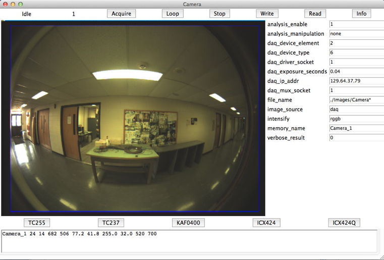
The Camera Instrument provides buttons for each of the image sensors it supports. Press one of these buttons and the Camera will be configured instantly for the sensor named on the button. See above for a list of image sensors supported by the Camera, and the values the configuration buttons will assign to various Camera parameters. Unlike the BCAM and Rasnik instruments, the Camera does not flash light sources. It takes pictures using ambient light only. There is no source device specified in the data acquisition parameters.
Note: To accommodate large differences in ambient light intensity, the Camera supports the anti-blooming and fast-move features of some TC255 and TC237 devices. Neither fo these features are used or required by the ICX424A image sensors. When the Camera is configured for these sensors, we enable anti-blooming with daq_anti_blooming, and we enable fast-move with daq_fast_move. By default, anti-blooming and fast-move are enabled for TC255 and TC237 sensors. When we use anti-blooming with a device that does not provide anti-blooming, the anti-blooming has no effect. When we use fast-move with a device that does not support fast-move, the result is a streaky, white image. The A2056 supports fast-move to readout both TC255P and TC237B image sensors. No other device supports fast-move. The A2056, A2051, and A2048 support anti-blooming.
The Camera allows us to read images from the daq, memory, or file, just like any other instrument. The Camera allows us to manipulate these images before it displays and analyzes them. We specify one or more manipulations in the analysis_manipulation string. By default, this string is "none". For a list of the manipulation codes and their functions, see lwdaq_image_manipulate. The Camera Instrument supports all manipulations available to lwdaq_image_manipulate that operate on only one image. The subtract and combine manipulations, for example, are not supported by the Camera. The "grad" manipulation, for example, returns an image of the magnitude of the intensity gradient in the original image. We specify multiple manipulations by listing their codes separated by spaces. The Camera will perform the manipulations consecutively and it will replace the original image with the final product. After performing whatever manipulations we specify, or after no manipulations at all, the Camera performs a simple analysis of the image by calling lwdaq_image_characteristics. The Camera result contains ten numbers.
Camera_1 20 3 343 243 73.3 15.5 121.0 48.0 244 344
The first four numbers are always integers, and they give the left, top, right, and bottom edges of the analysis boundaries. The next four numbers are real-valued. They are the average, standard deviation, maximum, and minimum intensity of the image within the analysis boundaries. The last two numbers are always integers. They give the height and width of the image.
The Diagnostic instrument provides an oscilloscope-like display of the power supply voltages on the driver board, and calculates the average current running out through each of them. The result string provides the power supply voltages and currents, the most recent device loop time, and other diagnostic parameters. The instrument is defined by Diagnostic.tcl. The instrument provides extra buttons that allow us to manipulate and test devices directly. When it acquires, the Diagnostic instrument reads the hardware, firmware, and software version numbers from the driver. As with any instrument, set verbose_result to 1 to get a description of the result numbers.
We change the voltage scale, offset, or coupling for the display by entering in new values in the entries dedicated to each of these variables. When we press return while in one of these entries, the display will refresh with the existing data. We change the seconds per division and the offset of the left edge from time zero (the time of the first sample). We can change the number of seconds per division for the display as well.
The Diagnostic result string contains fourteen numbers. Here they are listed as they are with verbose_result = 1 in the Diagnostic text box:
Software Version: 15
Hardware Type: 71
Hardware Version: 1
Firmware Version: 7
Most Recent Loop Time (ns): 125
Data transfer speed (kBytes/s): 105
+15V Supply Voltage (V): 14.743
+15V Supply Current (mA): 10.669
+5V Supply Voltage (V): 4.923
+5V Supply Current (mA): 30.103
-15V Supply Voltage (V): -14.804
-15V Supply Current (mA): 8.348
Commom Mode Gain (V/V): -0.0134
Differential Mode Gain (V/V): 66.0
The common and differential gain are properties of the differential amlifier that the LWDAQ Driver uses to measure its power supply voltages and currents. The most recent loop time will be valid if a loop job has been executed since the driver has been reset. The data transfer speed applies to the TCPIP connection between the driver and the data acquisition computer.
The A2037E and A2037A allow us to turn on and off the data acquisition power supplies. The Head Power On and Head Power Off buttons turn on and off the +5 V and ±15V power supplies to all multiplexers and devices connected to the driver we specify in the configuration entries. If we turn the head power off on our LWDAQ, everyone else will get no data from it until they realize what we have done, and turn the power back on again. If we want to turn the power off and then on again, wait for several seconds after turning the power off, to let the circuits settle in preparation for power-on reset. The Reset button resets the driver state machines, but not the devices. Some drivers turn off their data acquisition power supplies when we reset them, and others turn on their data acquisition power supplies. The behavior of our driver will depend upon its firmware version number.
The Sleep button sends to sleep the target device we specify with the config array entries. The Wake button wakes it up again. Because waking and sleeping are done automatically by all data acquisition instruments, we don't do any harm by sending a device to sleep. But we might bring down the LWDAQ power supplies if we wake up too many devices and forget to put them to sleep again. One way to put all devices attached to a driver to sleep is to use the Sleep All button. Another way to send all devices to sleep is to press the Head Power Off button, count to ten, and press the Head Power On button.
The Loop_Time button executes a loop job and returns the total propagation time for an electrical signal travelling to the target device and back again. The loop time for a working cable is 5.0 ns per meter of cable between the driver and the device, as shown in this graph.
The Transmit button transmits the commands we specify in hexadecimal to the target device. Enter a command, or a list of commands separated by spaces, in the command entry box next to the Transmit button, and press transmit. If we want the same single command transmitted multiple times in succession, enter a non-zero number in the repeat entry box. If we combine a list of commands with a non-zero repeat value, each command will be transmitted multiple times before the next command is transmitted multiple times.
The maximum value accepted by our driver's repeat counter depends upon the driver's firmware version. We can be confident, however, that we can go up to 65535 with any A2037E or A2037A.
Example: We want to turn on the front left laser on a Blue Azimuthal BCAM. Go to the Blue Azimuthal BCAM Head (A2048) Manual and look at its command bit allocation. We turn on the left laser with command 1080 hexadecimal. Enter "1080" in the box next to the Transmit button, select our BCAM with daq_driver_socket and daq_mux_socket and daq_driver_addr. Press the Transmit button. We should see our laser turn on and stay on. To turn it off and send the BCAM to sleep, transmit 0000.
The Diagnostic instrument allows us to execute any of its special button commands before it acquires power supply measurements, through the daq_actions parameter. We may also specify delays in milliseconds by adding an integer to this string. The following table relates the button we want to execute to the code word we include in the daq_actions string. We separate the code words with one or more spaces.
| Action | Button | Code Word |
|---|---|---|
| Send Target Devic to Sleep | Sleep | sleep |
| Send all Devices to Sleep | Sleep All | sleepall |
| Wake Target Device | Wake | wake |
| Measure Loop Time | Loop Time | loop_time |
| Transmit Hexadecimal Commands | Transmit | transmit |
| Head Power Off | Head Power Off | off |
| Head Power On | Head Power On | on |
| Reset LWDAQ Controller | Reset | reset |
| Delay of n milliseconds | no button | n |
Specify any number of the above code words in the daq_actions string, combined with any number of delays in milliseconds, and the Diagnostic instrument will execute them before it measures the driver power supplies.
Example: The string "reset off 1000 on 100" resets the controller, turns off the head power supplies, waits one second, turns on the power supplies, and waits for a hundred milliseconds.
By means of the daq_actions string, we can use the Diagnostic instrument to cycle the driver power supplies and check for devices that remain awake after the cycle. The delays allow us to make sure that the power supplies have a chance to turn off fully, and to turn on again.
In large LWDAQ systems containing devices with unreliable power-up reset, power supply cycling is essential to guarantee that all devices are in their sleep state and the power supplies are stable. We describe the power supply problems experienced by large LWDAQ systems in the Large Systems section of the LWDAQ Specification. To help us deal with these problems, the Diagnostic instrument can turn off and on the power supplies automatically, check the power supply voltages, and repeat the same cycle until it sees the power supplies turning on properly.
With daq_psc set to 1, the Diagnostic Instrument checks the power supply voltages before it completes data acquisition. The letters "psc" stand for "power supply check". If the power supplies lie within the ranges specified by the info array, acquisition ends. But if the supplies are out of range, the instrument acquires again. Acquisition will end when the power supplies are within range, or after psc_max_tries attempts. The power supply ranges are defined by elements in the info array. The maximum acceptable voltage for the +15V supply is max_p15. The minimum is min_p15. The +5V and −15V ranges are defined by max_p5, min_p5, max_n15, and min_n15. Note that we use "max" to mean "most positive acceptable value" and "min" to mean "least positive acceptable value".
Example: The string "off 1000 on 100" cycles the power supplies. With daq_psc = 1 and psc_max_tries = 4, the Diagnostic instrument cycles the power supplies up to four times to try to bring up the power supplies to their correct voltages.
The Dosimeter uses an image sensor to detect ionizing radiation, measure accumulated neutron dose, and find damaged pixels. The charge deposited in the image sensor pixels by ionizing radiation is a measure of ionizing dose. The dark current in the image sensor is a measure of accumulated neutron damage. The number of bright spots, or hits in the image, and their combined brightness, can be a measure of accumulated neutron dose or the current ionizind dose rate. The Dosimeter supports various ways to control pulsed radiation sources and mechanical shutters with LWDAQ commands. With the help of these controls, we can use the Dosimeter to take x-ray images with a pulsed x-ray source. We introduced the Dosimeter in Hit Counting. The instrument supports radiation detection with the TC255, KAF0400, TC237, ICX424 and ICX424Q image sensors. Use the buttons in the Info panel to configure the dosimeter for a particular sensor. The figure below shows a Dosimeter image taken with the TC255P.
All image sensors suffer cumulative damage from fast neutrons. This damage increases their dark current. Thus the image sensor dark current can be used as a measure of accumulated neutron dose. The dark current is also a strong function of temperature. A measurement of the dark current, combined with a measurement of the ambient temperature, provides us with an estimate of the cumulative fast neutron dose. The transfer array of an image sensor acts as general-purpose radiation counter. The TC255 and TC237 transfer array is an aluminum-masked array of pixels adjacent to the image array. The ICX424 transfer array is beneath the image array, also masked from light. The thin layer of silicon in the transfer array records electron-hole pairs generated by neutrons, photons, and charged particles. The KAF-0400 and KAF-0261 have no transfer array, so we must use the optical imaging area to detect ionizing radiation.
The Dosimeter can provide background subtraction during data acquisition. With daq_subtract_background = 1, the Dosimeter will take two images with the same exposure time and subtract their intensities. The Dosimeter will turn on a radiation source for the first image, and leave the source off for the second image. The difference between the two we can assume to be caused entirely by the radiation source. Even if the radiation source is continuous, the hits in the second image will generate negative values in the subtracted image, and these negative values will be cropped to zero. Only the hits in the first image will remain in the subtracted image. So long as the radiation charge is concentrated in a small fraction of all pixels, the background-subtracted image will provide a reliable measurement of dose rate.
The Dosimeter can provide gradient subtraction during analysis. With analysis_enable > 1, the Dosimeter first calculates the vertical intensity gradient within the analysis boundaries of the original image, then applies subsequent analysis to the image after it has been subjected to gradient subtraction with the "subtract_gradient" option of lwdaq_image_manipulate. The gradient-subtracted image has both its vertical and horizontal intensity gradient removed, and in such a way that the intensity of the top-left pixel in the analysis bounds remains unchanged. With analysis_enable = 3, the Dosimeter replaces the original image with the gradient-subtracted image and displays the gradient-subtracted image in the Dosimeter panel so we can see it. With analysis_enable = 2, we use the gradient-subtracted image for analysis, but do not display it or alter the original image in memory. With analysis_enable = 1, we use the original image for analysis.
The first number in the result string is the slope of intensity in cnt/row, calculated within the analysis bounds of the unmodified image. The slope of intensity from bottom to top of an image is proportional to sensor dark current. It is up to the user to convert counts per row (cnt/row) into counts per millisecond (cnt/ms) using a knowledge of the image sensor and the readout speed. The standard LWDAQ pixel readout proceeds at 2 MPSP, so we can get the time per row by dividing the number of pixels in the row by two million. For the TC255P, we have 174 μs/row. For the ICX424 we have 350 μs/row.
The second number is charge density, which has units of counts per pixel (cnt/px). We add the charge in all the hits in the analysis bounds and divide by the total number of pixels in the analysis bounds to obtain the charge density. The hits are contiguous collections of bright pixels. A bright pixel is one that is above a threshold, and the charge in a bright pixel is its intensity above a background intensity. We specify the background and threshold intensities with the analysis_threshold string, which works the same as in the BCAM Instrument. The threshold string also allows us to specify a minimum or a maximum number of pixels a hit can contain for it to be included in the charge density measurement. Only hits that meet the criteria specified in the threshold string will contrinute to the charge density.
The third number is the standard deviation of intensity in the analysis bounds. The fourth number is the threshold intensity we used to isolate the bright pixels. The fifth number is the total number of hits found in the image. After these five values, we may have one or more hits listed, as dictated by analysis_num_hits. If this parameter is zero, no hits will be listed. If this parameter is a positive integer, it gives the number of hits that will be listed in the remainder of the results string. If this parameter is "*", the analysis lists all valid hits in the image. The maximum number of hits the Dosimeter analysis will find is given by max_num_spots in spot.pas. By default, each hit in the list is represented by its total brightness above background. But if analysis_include_ij = 1, the column and row of the pixel closest to the optical center of the hit will be be appended to the brightness. Thus we might have "92 256 87" for one hit, meaning brightness 92, column 256 and row 87. If we have asked for more hits than are available, the non-existent hits will be represented by brightness −1 and location "0 0".
Neutrons will damage a small fraction of pixels far more than others, resulting in a constellation of bright pixels. When there are large bright spots in the image that are due to light rather than ionizing radiation or neutron damage, we can reject the optical spots with a suitable threshold string. Threshold string "20 & 2 <" instructs the dosimeter to use the median intensity as the background, set the threshold twenty counts above the backgrounmd, and accept only hits that contain no more than two pixels. Optical spots are always larger than two pixels.
During data acquisition, the Dosimeter clears charge out of the detection area and then activates or flashes a source of radiation. If daq_flash_seconds is greater than zero, the Dosimeter flashes a radiation source with a flash_job in the same way that the BCAM and Rasnik flash their light sources. We specify the source with a driver socket, element number, multiplexer socket and device type. The LWDAQ driver sends the activation command to the radiation source, waits for the specified length of time, and sends the de-activation command.
If daq_activate_hex is not equal to 0000, the Dosimeter activates a source of radiation with a single LWDAQ command word. We assume that the activated source will de-activate itself some time later, as specified by the value of the command word. The Dosimeter treats it as a hexadecimal representation of this sixteen-bit command word, and transmits it to the source device. Thus the Dosimeter can turn on a radiation source with a single command.
The Dosimeter is designed to either flash a radiation source or activate a source, but not both. If both flashing and activation are specified, the Dosimeter prints a warning message in its text window. Once activation or flashing is complete, assuming we specify one of them, the Dosimeter waits for daq_exposure_seconds before reading out the sensor image. An example of a radiation source that activates with a single command is the X-Ray Controller (A2060X). The A2060X uses the top eight bits of the command to determine its activation period, and deactivates itself.
The Flowmeter Instrument is defined by Flowmeter.tcl. It uses the RTD Head (A2053) to measure gas flow rate with a PT1000 platinum temperature sensor. The A2053 has a heater circuit that runs 15 mA through a PT1000 to heat it up, and then measures the time constant of its cooling to ambient temperature. In theory, the inverse of this time constant is proportional to the gas flow rate in kg/s around the sensor.
Figure: The Flowmeter Instrument on MacOS. The data is from the still-air platinum sensor. The green and red lines should coincide in an accurate flowmeter measurement, but they do not for sensors in still air, because cooling through the sensor leads is significant compared to cooling in the air.Select a sensor for flow measurement in the same way we select a sensor in the Thermometer instrument. There are eleven sensor inputs on the A2053, selected with the daq_sensor_element variable. The flowmeter measurements takes about ten seconds with the default instrument settings. In the first second, it measures the ambient temperature of the gas. In the next two seconds, it heats up the sensor. For the seven seconds after that, it records the temperature of the sensor. When all the data has been transferred to the LWDAQ Driver, the Flowmeter displays it on the screen, and uses the last six seconds of the cool-down to calculate the time constant. The Flowmeter ignores the first second of cool-down after the end of the heating, because secondary time-constants manifest themselves during this first second, and degrade the accuracy of our measurement.
If we change the Scale (s/div), we change all the seconds in the above paragraph to time periods equal to the new value. The only exception is the heating time, which is set independently with the daq_heating_seconds parameter.
After a Flowmeter acquisition, we need to wait a few more time constants before we acquire again: the sensor needs to cool down completely to ambient temperature. We will see in the display two red graphs. One is a linear plot of the temperature. It is curved. The other is a log-linear plot of temperature, and this plot extends only across the final six divisions of the display. In green is the straight-line fit to the log-linear graph, which we transfer also into the linear plot so we can compare the actual temperature with the fitted-temperature curve.
The Flowmeter output is the inverse time constant (1/s), the rms residual from the fit (C), the ambient temperature (C), the temperature at the start of the measurement fit (C above ambient), and the temperature at the end (C above ambient). We obtain better than 0.03% resolution in inverse time constant with constant laminar flow in a pipe, and we observe that the inverse time constant increases by roughly 1% for a 3% increase in gas flow. The curve of inverse time constant versus flow rate must be measured, because it is not exactly linear. We have an electronically-driven proportional valve connected to our apparatus, and we can calibrate a sensor in five minutes automatically.
The Gauge measures physical quantities such as temperature, resistance, or strain using a two-point calibration of a linear measuring device such as the Resistive Sensor Head (A2053). The Gauge Instrument is almost identical to the Thermometer, except it does not assume that the unit of the quantity you are measuring is Centigrade. The Gauge Instrument is defined by Gauge.tcl.
The Gauge measures the bottom and top reference voltages returned from an A2053 or compatible device. You specify values for bottom_ref_y and top_ref_y that correspond to the underlying physical quantities that give rise to the bottom and top reference voltages. Suppose you are using a Strain Gauge Head (A2053S) with bottom reference resistance 115Ω and top reference resistance 125Ω. You enter 115 for ref_bottom_y and 125 for ref_top_y in the Gauge config array. When you acquire data from channels on the A2053S, the Gauge will return the resistance across each channel you acquire from. The Gauge measures the resistance by drawing a straight line through the voltage it reads from the bottom and top reference resistors, and using this straight line to determine the resistance corresponding to the voltage it reads back from other channels.
The Gauge takes daq_image_width samples of each voltage it measures. By this means, it obtains daq_image_width measurements of an underlying physical quantity. With analysis_enable > 0, the Gauge plots these individual measurements in its display rectangle. With analysis_enable = 1, the Gauge result string contains the average of these daq_image_width measurements for each channel you specify. With analysis_enable = 2 , the Gauge returns the average and the standard deviation of the measurements.
If you want to measure temperature with a 100-Ω RTD using the A2053S, and you want the Gauge to convert RTD resistance into temperature, enter the RTD temperature that corresponds to an RTD resistance of 115Ω in the ref_bottom_y box, and the resistance that corresponds to 125Ω in the ref_top_y box. These temperatures are 38.96°C and 64.94°C respectively. Now the Gauge will convert resistance into temperature for you in its results line.
If you want to measure strain with a 120-Ω strain Gauge using the A2053S, and the Gauge factor of the strain Gauge is 2.0, enter -20800 for ref_bottom_y, indicating -20800 ppm strain, and +20800 for ref_top_y, indicating +20800 ppm strain. The Gauge will convert the strain Gauge's resistance into ppm strain in its results line.
You can, of course, connect both RTDs and strain Gauges to the same A2053S, and you can read them all out in one acquisition. The Gauge will not convert some channels into temperature and others into strain. It does either temperature or strain or resistance or some other units. We leave it to you to decide if you want to convert resistance to temperature and strain yourself, or if you want to configure and acquire from the Gauge Instrument once for your temperature sensors and a second time for your strain Gauges.
We also note that the Gauge will work equally well with the RTD Head (A2053A) and 1000-Ω RTDs. The A2053A uses 1060 Ω and 1100 Ω for its bottom and top reference resistances. You enter 15.38°C for ref_bottom_y, and 25.69°C for top_ref_y, and the Gauge will convert your 1000-Ω RTD measurements into degrees centigrade.
The Gauge's measurement method is accurate so long as the voltage returned by the measuring device is linear with the physical quantity it measures. All versions of the A2053 are designed so that they are linear to within 100 ppm of their dynamic range.
The Inclinometer, also called a tilt sensor, measures inclination in two directions using a liquid level sensor with five electrodes. The Inclinometer Instrument is defined by Inclinometer.tcl.
The Inclinometer Instrument works with the Inclinometer Head (A2065) and Inclinometer Sensor Head (A2066). The A2065 is a LWDAQ Device with programmable logic and analog circuits to drive the liquid level sensor. The A2066 holds the liquid level sensor and connects to the A2065 via a six-way flex cable. For a picture of the two of them in a box, see here.
The sensor has five electrodes. Four lie upon the corners of a square. The fifth lies in the center of the square. We call that one CTR in the circuit diagram. Two electrodes on opposite corners we call X+ and X−. The other two we call Y+ and Y−. In the Operation section of the Inclinometer Head Manual we describe how we measure the tilt of the sensor in the X and Y directions. There you will also find a description of the elements returned in the Inclinometer Instrument result.
A Rasnik Instrument takes an image of a chessboard pattern and determines the point in the chessboard projected onto a reference point in the image sensor. Our Rasnik Instrument is defined by Rasnik.tcl. The NIKHEF laboratory in the Netherlands invented the Rasnik Mask, which is a chessboard with some squares switched from black to white, and other switched from white to black in such a way as to indicate to a camera which part of the mask it is looking at, even though the camera sees only a small portion of the mask.
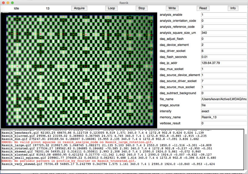
We configure the Rasnik Instrument for a particular image sensors using the image sensor buttons in its Info panel. The ICX424 button, for example, configures the instrument for the ICX424. By default, the Rasnik Instrument is configured for the TC255. (When we switch between ICX424 and ICX424Q readout, however, the Rasnik Instrument does not, as yet, set parameters analysis_add_x_um and analysis_add_y_um as it should to make the rasnik measurement independent of the readout.)
We configure the Rasnik Instrument for a particular light source using daq_source_device_type in the Info panel. By default, the Rasnik is configured to operate with a source of device type = 1 (LED), which is correct for single-mask devices such as the Proximity Mask Head (A2045). Change the value of daq_source_device_type to operate with other device types, as for the BCAM Instrument.
We distinguish between the magnification of the mask in the x (horizontal) and y (vertical) directions. You can see a Rasnik result in the figure above. The name at the beginning of the result is the name of the image file we analyzed, or if we captured the image from the LWDAQ, it is the name of the image in the LWDAQ image list. We have lwdaq_rasnik as a command-line routine in TclTk, lwdaq_image_create, and so on. If we specify an image in the LWDAQ image list, then the name of this image is the name at the beginning of the rasnik result.
| Index | Parameter |
|---|---|
| 0 | image of file name |
| 1 | mask x-coordinate in microns |
| 2 | mask y-coordinate in microns |
| 3 | image x-direction magnification |
| 4 | image y-direction magnification |
| 5 | rotation of pattern in image |
| 6 | estimated precision in microns |
| 7 | rasnik square size in microns |
| 8 | pixel size, assumed square, in microns |
| 9 | orientation code |
| 10 | image sensor reference point x-coordinate in microns |
| 11 | image sensor reference point y-coordinate in microns |
| 12 | skew in x-direction in milliradians per millimeter |
| 13 | skew in y-direction in milliradians per millimeter |
| 12 | slant in milliradians |
The first and second numbers are the coordinates in the rasnik mask of the point in the mask that is projected by the rasnik lens onto the reference point in the CCD. The reference point does not strictly speaking have to lie within the CCD. It is a point in "image coordinates". Unlike the mask coordinates, which are right-handed, and proceed from the bottom-left corner of the mask, the image coordinates are left-handed, and proceed from the top-left corner of the top-left pixel in the image. Positive x is left to right, and positive y is top to bottom. We can specify image coordinates in microns, or in pixels. Within the analysis library, we use pixels for the most part, but when you specify the reference point yourself, as you can in the LWDAQ_info_Rasnik array, you do so in microns.
Rasnik_large.gif 69781.76 77644.95 4.059326 4.040204 9.731 0.686 120.0 10.0 3 3450.0 2500.0 -0.343 -0.813 -4.992
The third and fourth numbers are the x and y direction magnifications. The x and y directions we refer to here are not those of the image coordinates, but rather of what we call "pattern coordinates". The pattern coordinates are parallel to the mask squares. The x-direction is roughly left-to-right along the squares, and the y-direction is roughly top-to-bottom.
The fifth number is the rotation of the pattern coordinates with respect to the image coordinates, and so we can refer to it as the mask rotation. Positive rotation is anti-clockwise rotation of the image with respect to the CCD, or clockwise rotation of the mask when we look from behind the mask towards the CCD through the lens.
The sixth number is an estimate of the accuracy of the mask x and y measurement. We have improved this error estimate so that it now includes the error we get from using a reference point that is displaced from the center of the area in the image we use to determine the rasnik measurement. We call this area the "analysis_bounds". When we use the top-left corner of the image as our reference point (coordinates 0, 0), our measurement is less accurate than if we use the center of the analysis bounds. This is because there is a stochastic error in our measurement of the rotation of the mask, and we must multiply this error by the distance from the center of the analysis bounds to the reference point to obtain the additional error caused by this displacement. That is not to say, however, that we lose anything by using the top-left corner. We provide a TclTk command line routine lwdaq_rasnik_shift which allows you to convert a rasnik measurement from one reference point to another, and in doing so you can remove the rotation error. In the following example, we use lwdaq_rasnik_shift to shift a rasnik reading to coordinates (1, 2) in millimeters. The result will give the Rasnik measurement with respect to the new reference coordinates in the CCD.
set result [LWDAQ_acquire Rasnik]
Rasnik_slanted.gif 28603.44 17241.51 1.612901 1.216688 -11.342 0.580 120.0 10.0 1 3500.0 2600.0 -0.005 -7.275 -39.127
lwdaq_rasnik_shift $result -reference_x_um 1000 -reference_y_um 2000
Rasnik_slanted.gif 27047.94 17717.04 1.612901 1.216688 -11.342 0.580 120.0 10.0 1 1000.0 2000.0 -0.005 -7.275 -39.127
The seventh number is the size of the squares in the rasnik mask, in microns, as provided by analysis_square_size_um. The square sizes we have used are 85, 120, 170, and 340 μm. The eighth number is the size of the pixels, in microns, as provided by analysis_pixel_size_um. Note that we assume the pixels are square, which has been the case for all the image sensors we have used in rasnik instruments.
The ninth number is the orientation code. Here are the names of each numerical orientation code, as they appear in rasnik.pas.
rasnik_mask_orientation_nominal=1;
rasnik_mask_orientation_rotated_y=2;
rasnik_mask_orientation_rotated_x=3;
rasnik_mask_orientation_rotated_z=4;
The x, y, and z axes we refer to in the names above are axes in the mask coordinates, with z being out of the mask. The mask has a nominal orientation, in which the x code increases from left to right as seen from the front of the mask, and the y code increases from bottom to top. If we rotate the mask by 180° about the y-axis, the x-code will decrease from left to right, and the code squares will be in reverse order. The y-code, however, remains unaffected. The mask is in orientation 2. If we rotate by 180° about the x-axis instead, the y-code will decrease from bottom to top, and the code squares will be in reverse order. The x-code will be unaffected. The mask is in orientation 3. If we rotate by 180° about the z-axis, both the x and y code squares will be in reverse order. The x-code will decrease from right to left and the y-code will decrease from bottom to top. The mask is in orientation 4.
There are other rotations of the mask from its nominal position, such as 90° around the x-axis or 270° about the z-axis, but each of these other rotations is equivalent to one of our four defined orientations, so we do not bother to define them as separate orientations in our code. We do have one last orientation code.
rasnik_try_all_orientations=0;
This orientation code never appears in the rasnik output, but you can specify it as an input to the rasnik analysis, in which case the analysis will try all orientations and pick what it thinks is the best one.
The tenth and eleventh numbers are the reference point the rasnik analysis used, specified in microns from the top-left corner of the top-left pixel. The Rasnik Instrument uses analysis_reference_code to determine how it should choose the reference point for analysis. The default value of the reference code is zero.
| Code | Function |
|---|---|
| 0 | Use top-left corner of top-left pixel. |
| 1 | Use center of analysis bounds. |
| 2 | Use center of image sensor. |
| 3 | Use analysis_reference_x_um and analysis_reference_y_um. |
The reference_x_um and reference_y_um parameters are available in the Info panel. We prefer to use reference code 2, to select the center of the image, where errors in our measurement of the rotation of the mask pattern have the least effect upon our calculation of the point in the mask that is projected on to the reference point. Nevertheless, we often use reference code 0, which has the advantage of being a point in the image whose location is independent of pixel size and sensor width. To specify an arbitrary reference point, we use a coordinate system in units of microns with its origin at the top-left corner of the top-left pixel in the image. By "image" we mean the array of pixels we display in the Rasnik Instrument, and which we can store to disk. The image contains all pixels available from the image sensor, as well as extra columns on the left and one or more extra rows on the top. The top-left pixel in the image does not exist in the image sensor at all, but is produced by our data acquisition system while we get ready to read out the first row of the sensor. In any case: the top-left corner of the top-left pixel is location (0 μm, 0 μm). The x-axis runs from left to right across the image and the y-axis runs from top to bottom. A TC255P image has 344 columns and 244 rows. The pixels in the sensor are 10 μm square. The center of the image is (1720 μm, 1220 μm). The following table gives the center-point and pixel size for various LWDAQ image sensors.
| Sensor | Pixel Width (μm) | Center X (μm) | Center Y (μm) | Columns | Rows |
|---|---|---|---|---|---|
| TC255 | 10 | 1720 | 1220 | 344 | 244 |
| KAF0400 | 9.0 | 3600 | 2340 | 800 | 520 |
| TC237 | 7.4 | 2553 | 1850 | 690 | 500 |
| ICX424 | 7.4 | 2590 | 1924 | 700 | 520 |
| ICX424Q | 14.8 | 2590 | 1924 | 350 | 260 |
| KAF0261 | 20 | 5200 | 5200 | 520 | 520 |
The analysis boundaries are not included in the Rasnik output. Your DAQ script can get the analysis bounds from the lwdaq_image_characteristics command.
Rasnik_slanted.gif 81043.08 48850.95 0.421252 0.317770 -11.342 1.642 340.0 7.4 1 2590.0 1924.0 -0.007 -9.832 -39.127
The twelfth and thirteenth numbers in the Rasnik Instrument output string are the skew of the image in the x and y directions. When the mask magnification increases from left to right, the horizontal lines in the pattern will diverge. We express this divergeance as the rate at which the horizontal line slope changes in radians per meter from left to right, and we call this the x-direction skew. The y-direction skew is the rate at which the slope of the vertical lines changes from top to bottom. Note that radians/meter = mrad/mm, so we use these interchangeably.
The fourteenth parameter is the image slant in milliradians. The slant is the amount by which the mask's vertical and horizontal edges are not perpendicular at the center of the analysis boundaries. We look at the lower-right quadrant created by the intersection of a vertical and horizontal edge near the center of the analysis bounds. The amount by which the internal angle of this lower-right quadrant is less than π/2 is the slant.
The Rasnik Instrument's analysis_disable_skew parameter turns off the measurement of skew and slant by forcing both parameters to zero during image analysis. When we know the slant and skew of an image are near zero, but the image is corrupted with dirt, we will do better by forcing the slant and skew to zero so that we can apply the rasnik analysis many times to the image until we arrive at a successful fit. Here we have the result of analyzing our very-skewed image with skew enabled and disabled. In order to obtain a result with skew disabled, we had to allow random bounds and multiple applications of the analysis.
Rasnik_very_skewed.gif 26719.23 19364.18 0.929639 1.316329 1.576 0.410 120.0 10.0 1 3500.0 2600.0 -8.022 -0.703 -1.422
Rasnik_very_skewed.gif 26703.00 19386.65 0.908387 1.329073 18.014 2.093 120.0 10.0 1 3500.0 2600.0 0.000 0.000 0.000
The Rasnik provides automatic flash time adjustment and background subtraction, just like the BCAM, controlled by daq_adjust_flash in the Rasnik Panel. The Rasnik extended acquisition adjusts the exposure time in the same way as the BCAM's extended acquisition. But the Rasnik's extended acquisition does not adjust its analysis boundaries. The Rasnik allows you to specify a separate IP address for the source device LWDAQ, through the daq_source_driver_addr parameter, just like the BCAM.
As you select different reference codes, we mark the reference point in the Rasnik Panel different ways. If you set show_fitting to 1 you will see the steps of our rasnik analysis in the derivative images. If you set show_fitting to 1000 the program waits for 1000 ms between its displays of intermediate steps. If you set show_fitting to -1, the program will put up a little window with an OK button, right over the main window, and you press the button to continue. If you perform live capture with the -1 option, you can get a bit stuck trying to get to the Stop button after the OK button. Use the apple-t key on MacOS X, or control-t on Linux, to stop all instruments.
By setting analysis_enable to 0, you can disable the Rasnik's image analysis. This stops the Rasnik drawing its colored lines over the image. By setting analysis_enable to numbers greater than 1, you enable enhanced versions of the image analysis. In particular, you enable the Rasnik Instrument's boundary adjustment process.
| analysis_enable | analysis sequence |
|---|---|
| 0 | no analysis, no drawing |
| 1 | one analysis attempt, overlay result |
| 2 | multiple attempts with boundary adjustment, overlay final result |
| 3 | multiple attempts with boundary adjustment, overlay intermediate and final result |
| 10 | no analysis, no drawing |
| 11 | smooth twice with 3×3 box filter, proceed as (1) |
| 12 | smooth twice with 3×3 box filter, proceed as (2) |
| 13 | smooth twice with 3×3 box filter, proceed as (3) |
| 20 | no analysis, no drawing |
| 21 | smooth with 3×3 box filter, shrink by ×2, proceed as (1) |
| 22 | smooth with 3×3 box filter, shrink by ×2, proceed as (2) |
| 23 | smooth with 3×3 box filter, shrink by ×2, proceed as (3) |
| 30 | no analysis, no drawing |
| 31 | smooth with 3×3 box filter, shrink by ×3, proceed as (1) |
| 32 | smooth with 3×3 box filter, shrink by ×3, proceed as (2) |
| 33 | smooth with 3×3 box filter, shrink by ×3, proceed as (3) |
| 40 | no analysis, no drawing |
| 41 | smooth with 3×3 box filter, shrink by ×4, proceed as (1) |
| 42 | smooth with 3×3 box filter, shrink by ×4, proceed as (2) |
| 43 | smooth with 3×3 box filter, shrink by ×4, proceed as (3) |
With analysis_enable set to 2, the Rasnik tries to analyze a portion of the original analysis bounds. It selects a smaller analysis rectangle at random within the original rectangle. The minimum width and height of this new rectangle is analysis_min_width, in units of pixels. If this alternate rectangle produces a valid rasnik result, the analysis terminates and returns this result. Otherwise, the analysis routine writes one or two lines of red error messages to the instrument panel and then tries another rectangle. It keeps trying until it reaches analysis_max_tries or it meets with success. If it is successful, the analysis draws the rasnik measurement on the image.
At the end of the bounds-adjusting analysis, the analysis boundaries in the analyzed image will be set equal to the rectangle within which the analysis obtained a valid result. If it does not obtain a valid result, it leaves the original boundaries of the image intact. You can find out what the final analysis boundaries were with the help of lwdaq_image_characteristics applied to image memory_name. If you want to know how many boundaries the analysis tried before it completed or aborted, you can check the analysis_index_tries parameter in the instrument's info array.
When analysis_enable, the analysis follows the bound-adjusting algorithm, but displays each rectangular boundary on the screen as it goes. This display is entertaining when you are working directly on the machine performing the analysis, but if you are connected to via X-Windows, you will find the rectangle-drawing slows the Rasnik Instrument down.
The Rasnik Instrument will perform various manipulations upon the acquired image before analysis begins. We can smooth the image twice with a 3×3 box filter, which greatly attenuates the amplitude of stochastic and quantization noise (see lwdaq_image_manipulate). Alternatively, we can smooth once and then shrink the image by a factor of two for analysis. Even though the image we analyze has been shrunk, the results of analysis will apply to the original image. The Rasnik Instrument scales the pixel dimensions by two, and even adjusts the display zoom so that intermediate images will be displayed the same size as the original. Shrinking the image by a factor of two accelerates computation time. We can also shrink by a factor of three or even four.
The rasnik analysis can find patterns such as vertical bars, or an image of wire mesh. But such patterns have no code squares. With the analysis_pattern_only, we instruct the analysis to stop before it attempts to find code and pivot squares, and instead report the position, pitch, and orientation of the chessboard pattern in dimensions of pixels.
screen.gif 368.347 257.209 34.467 34.326 31.752 0.401 11
The result string contains seven numbers. The first two are the image coordinates of the top-left corner of one of the squares in the pattern. The coordinates are in units of pixels, not microns. Position (0, 0) is the top-left corner of the top-left pixel of the image. x and y coordinates of the pattern origin. The origin the image coordinates of the top-left corner of one of the squares in the chessboard. The next two numbers are the width of the squares in the near-horizontal direction and their width in the near-vertical direction. Units are again pixels. The rotation is counter-clockwise in milliradians. The error is an estimate of the fitting accuracy in pixels. The extent is the number of squares from the image center over which the pattern extends.
As we describe in Large Rotations, the Rasnik Instrument can analyze rasnik images rotated at any angle with respect to the image rows, provided we know approximately what the angle is in advance. As we rotate the rasnik mask within the image, the rasnik analysis will calculate the rotation. When the rotation exceeds one square divided by the image width, however, the rasnik analysis will fail. When we have a mask with a nominal rotation that is larger than the tolerance of the rasnik analysis, we can include this rotation in the analysis_rotation_mrad parameter. If the nominal rotation of the mask is 45° counter-clockwise, we enter 785 for the nominal rotation. The Rasnik Instrument rotates the image clockwise by the nominal rotation before analyzing. It must use a smaller analysis boundary because of lost regions on the rotated image, but it should be able to analyze the mask. The final rasnik measurement includes the nominal rotation plus the rotation measured by analysis in the unrotated image.
The Receiver Instrument is defined by Receiver.tcl.
Figure: The Receiver Instrument on MacOS.The Receiver Instrument operates with the Data Receiver (A3007). The Neurorecorder Tool uses the Receiver to obtain data from implanted telemetric devices such as the Subcutaneous Transmitter (A3013). Both the software and the hardware were developed by Open Source Instruments Inc. For more information, see the Receiver Instrument User Manual.
The RFPM Instrument is defined by RFPM.tcl.
Figure: The RFPM Instrument on MacOS.The RFPM (Radio Frequency Power Meter) Instrument operates with the RF Spectrometer (A3008). Both the software and the hardware were developed by Open Source Instruments Inc. The Spectrometer Tool uses the RFPM to obtain power measurements for its radio-frequency spectra.
The Terminal Instrument is defined by Terminal.tcl. Its purpose is to communicate with a LWDAQ device such as the RS-232 Interface (A2060C). It provides a console-like interface with a LWDAQ data device. During a data acquisition cycle, the Terminal sends a string of bytes to the device and downloads a string of bytes that it expects to receive in return. We use the Terminal with the RS232 Interface (A2060C) and the ADC Tester (A2100).
The Terminal composes a transmission string from four different sources, any one of which can be empty. First is a header, which we specify in tx_header. You specify bytes in tx_header by entering their decimal values separated by spaces. If you type "65" you specify the byte with ASCII value "A". If you enter "65 66", you specify "AB". If you enter "10 13", you get line-feed (LF) followed by a carriage-return (CR). After the header comes tx_ascii, in which you enter ASCII characters directly. If you type "A", you specify the byte with decimal value 65. After the ASCII string comes the contents of the file named in tx_file. If this string is empty, we skip the file contents. The final part of the transmission string is tx_footer, which we define in the same way as tx_header.
The Terminal sends tx_string to the target device one byte at a time. For each character, the Terminal sends a command word with the upper byte containing the character value and DRX (DC6) set to 1, as required by data devices during read jobs.
Example: The RS232 Interface (A2060C) transmits each character it receives over its RS232 interface.
Example: The ADC Tester (A2100) receives each byte as an instruction, which it executes immediately.
You use tx_header and tx_footer to send terminator characters at the end of a character string.
Example: We want to send commands to a motor controller over an RS-232 connection. We use the Terminal Instrument and the RS-232 Interface (A2060C). The A2060C cannot receive characters when it is transmitting. We set tx_header to "19" so as to begin our transmission with an XOFF character. This stops the controller from sending any bytes to the A2060C. We set tx_ascii to "<01 H16", which is the ascii string that selects controller number one and gives it the command to output all its settings. As a footer we send "13 10", which is CRLF. The CRLF tells the controller to start work. The Terminal composes the string and sends it to the A2060C as a sequence of device commands, using the top eight bits of each device command to hold the byte values. When the transmission is complete, the Terminal puts the A2060C in its receive state. The A2060C always transmits an XON character (decimal 17) when it moves into its receive state, and this lets the controller know that it can send its own data. The screen shot above shows the Terminal set up for this exchange.
The following table gives the decimal and hex values of some common control characters.
| Character | Description | Decimal | Hex |
|---|---|---|---|
| ETX | End of Text | 3 | 03 |
| EOT | End of Transmission | 4 | 04 |
| LF | Line Feed | 10 | 0A |
| FF | Form Feed | 12 | 0C |
| CR | Carriage Return | 13 | 0D |
| XON | Transmission On | 17 | 11 |
| XOFF | Transmission Off | 19 | 13 |
After sending the transmit string to the target device, the Terminal downloads a response string from the target device. It obtains the response string by consecutive byte transfers. The string will be rx_size bytes long, and will be stored in rx_string. If rx_size is zero, the Terminal skips the download, sets rx_string to an empty string, and ends its acquisition. The consecutive byte transfers cease when rx_size bytes have been received, or when the transfers from the target device end with the receive terminator character, whichever occurs first. We define the receive terminator character with rx_last. We set rx_last equal to the decimal value of an ASCII character. The value 0, which indicates the NULL character, has a special meaning: the Terminal does not look for a terminator character, but instead waits until the driver has received rx_size bytes from the target device.
Example: You connect a PC to the LWDAQ through an RS232 Head (A2060C). You transmit text lines to the PC terminated by FF characters, and a receive text lines terminated by FF charcters also. The longest answer you expect to receive is a few thousand characters, so you set the rx_size to 10000. You put your text instructions in tx_ascii. You set tx_footer to 12. You leave tx_file_name and tx_header empty. You set rx_last to 12. Suppose the PC is asking the questions. Set tx_ascii to the empty string and acquire. Wait until you have receive a string from the PC. The string should appear in the Terminal text window. Type your answer to the PC in tx_ascii. Acquire again, and so on. You could equally well set up the communication so that the Terminal was asking the questions. You send a query string and wait for the PC to answer.
The Terminal allows you to set a time-out for reading from the target device. The timeout applies only when waiting for a receive terminator character from the target device. The Terminal will give up waiting for the terminator after rx_timeout_ms and download rx_size bytes from the driver.
Once it obtains its rx_size bytes from the driver, the Terminal displays them in its image display area. Each byte appears as the gray-scale intensity of one pixel. The first byte is the first pixel in the second row (not the first row). With zoom set to 1, the pixels will be small. The default value of zoom for the Terminal is 2.
After it displays the data as gray-scale pixels, the Terminal analyzes the data and creates its result string. The result string depends upon the value of analysis_enable.
| analysis_enable | analysis |
|---|---|
| 0 | No analysis, results string is empty. |
| 1 | Result string is bytes received up to first terminator character. If terminator is NULL, result is equal to the all bytes received. |
| 2 | Result string is a list of signed one-byte decimal values separated by spaces. All bytes up to first terminating character are listed. If terminating character is NULL, all bytes are listed. |
| 3 | As 2, but result string is a list of unsigned one-byte decimal values separated by spaces |
| 4 | As 2, but result string is list of hex characters. |
| 5 | As 1, but remove all bytes zero and greater than 127 to enable printing. |
If the block of received bytes is large, or contains many non-standard ASCII values, you can work with the data in the Terminal image, using routines like lwdaq_data_manipulate.
[21-NOV-23] The Silhouette Camera (SCAM) instrument obtains images from the cameras of a Contactless Position Measurement System (CPMS). These cameras work with infrared backlights to obtain silhouette images of highly-reflective metallic objects. The SCAM instrument obtains an image from a camera while a backlight flashes.
To distinguish between silhouette and backlight, the SCAM applies an intensity threshold to the image. Anything below the intensity threshold is silhouette. The SCAM analysis marks all silhouette pixels in orange and leaves the others unmarked. In the example above, we see the entire silhouette colored orange. The first number in the SCAM result string is the number of silhouette pixels. The next two numbers are the minimum and maximum intensity in the image. The fourth and final number is the intensity threshold the analysis used to identify silhouette pixels.
To determine the silhouette intensity threshold, the SCAM uses the analysis_threshold string, which behaves in the same way as in the BCAM instrument. The threshold string "10 %", for example, sets the intensity threshold at a value 10% of the way from the minimum to the maximum image intensity. If the minimum intensity is 49 and the maximum intensity is 124, the threshold will be 56.5. Any pixel with intensity 56 or lower will be silhouette. Any with intensity 57 or higher will be background.
The SCAM's Info Panel provides buttons to configure the SCAM for common image sensors and light sources.
The Thermometer instrument allows you to measure temperatures from either a Bar Head (A2082), Bar Head (A2044), an RTD Head (A2053), or a WPS Head (A3022). these devices are equipped with platinum RTDs (resistance temperature devices). We tend to use the 1000-Ohm variety, with reference resistors 1060 Ohms and 1100 Ohms on the board to act as references for temperatures 15.38 C and 25.69 C respectively. The Thermometer Instrument is defined by Thermometer.tcl.
You tell the Thermometer which device you are using with the daq_sensor_name variable in the config array, which you can set to "A2082", "A2053", "A2044", or "A3022" (no spaces on either side of your entry). The A2082 and A2044 provide four RTD inputs, numbered 1 through 4, and the A2053 provides eleven, numbered 1 through 11. You specify which sensors you want to read, and the order in which you want to read them, using daq_sensor_element. In our default setup, the Thermometer reads out all eleven channels from an A2053, as well as the on-board bottom temperature reference and top temperature reference. We use numbers to select the sensors, the letter "B" to select the bottom reference resistor, and "T" to select the top reference resistor.
Connector P1 on both the A2044 and A2053 carries sensor elements 1 through 4. The connector has eight pins, with pin 1 being marked on the silk screen. The first two pins are for sensor 1, and so on. On the A2053, connector P2 carries sensors 5 through 8 in the same way. Connector P3 is a four-way connector and carries sensors 9 and 10. Sensor 11 is on P4, which is a two-way header that we usually leave out, so you can solder wires into the board if you want to.
The Thermometer measures temperature by comparing the resistance of every sensor you tell it to look at to the resistances of the bottom and top reference resistors. If you tell the Thermometer to measure the temperature of the bottom reference resistor, it goes through the same procedure, but instead of selecting an external sensor, it selects the bottom reference resistor. The bottom reference resistor should give you a temperature equal to ref_bottom_C in the info array.
For each sensor element, the Thermometer selects the bottom reference resistor, the sensor resistor, and the top reference resistor in turn. For each of these three resistors, if records a series of sixteen-bit ADC samples. The number of samples it records is equal to daq_image_width. When the Thermometer calculates the sensor temperature, it does so using the average of each of the three series of samples. The Thermometer writes the temperatures it measures to its results string, in the order you specify in daq_sensor_element.
The Thermometer takes daq_image_width samples of each voltage it measures. By this means, it obtains daq_image_width measurements of temperature. With analysis_enable > 0, the Thermometer plots these individual measurements in its display rectangle. With analysis_enable = 1, the Thermometer result string contains the average of these daq_image_width measurements for each channel you specify. With analysis_enable = 2 , the Thermometer returns the average and the standard deviation of the measurements.
The Thermometer display looks like an oscilloscope. It displays the individual temperature measurements that go into making the average measurement that the Thermometer writes to its result string. Each point displayed in the oscilloscope graphs is a sixteen-bit measurement of sensor resistance combined with the average bottom and top temperature measurements taken immediately before and after the sensor samples. You can zoom in on individual sensors, and expand the time scale using the numerical text entries below the display.
When the Thermometer acquires a new measurment, it determines its sixteen-bit ADC sample rate by looking at the "Scale (s/div)" entry below the oscilloscope, which is equal to display_s_per_div. The thermometer knows how many columns there are in the display per display division, and divides display_s_per_div by the number of columns per division to obtain the sample period. If the sample period required to conform to this rule is less than the smallest sample period possible with the driver's sixteen-bit ADC, then the Thermometer simply sets the period equal to this smallest value. Either way, the Thermometer knows the actual sample period, and displays the samples accurately along the time scale.
The Viewer allows us to mix data acquisition and analysis between two different instruments. It allows us to adjust the analysis boundaries, dimensions, and result string of an image. It will translate batches of images between DAQ and GIF image formats. The Viewer is defined by Viewer.tcl. The Viewer has no data acquisition parameters of its own. If you enter "daq" for image_source you will receive an error message.
When we double-click on an image pixel in any other instrument, the Viewer will display the region around the pixel. With zoom greater than one, this region is expanded so that it becomes a close-up view. We can then analyze the closeup with the analysis procedure of any other instrument, or we can save the closeup to disk. The Viewer's Acquire button causes the Viewer to read an image from disk or acquire an image using the acquisition procedure of another instrument. Its Analyze button applies the analysis of another instrument to the file it is displaying. The Read and Write buttons behave as they do for all instruments.
When we move the mouse over the image, the Viewer displays the column and row of the pixel under the mouse cursor in the "col" and "row" entries. Column zero is the left-most column and row zero is the top-most row. By control-clicking on the image and dragging, we can define new analysis boundaries. We can apply these boundaries to the existing image with Set Bounds, or we can instruct the Viewer to use our own bounds on all images it analyzes, whether they come from a file or another instrument, with Use These Bounds. You select which instrument's analysis procedure you want to apply with anslysis_source. If you want to read images from disk, set image_source to "file". If you want to acquire images from another instrument, enter the instrument name (with capital letters) for image_source.
Example: You want to analyze a batch of imags on disk to look for bright pixels in a particular rectangular region of the images. Set the analysis source in the Viewer to Dosimeter and configure the Dosimeter Instrument to find bright pixels. Open one image with the Viewer and define your rectangular region with the mouse. Check Use These Bounds. Press Acquire and select all files you want to analyze. The Viewer will analyze all of them, applying your particular region to each before calling the Dosimeter analysis, then printing the result to the Viewer text window.
The Viewer allows you to change the dimensions, analysis bounds, and results string of an image using the buttons and entry boxes. Enter your new values in the entry boxes and press the appropriate button. The "−1" default values for analysis boundaries tell the Viewer to leave pre-existing boundaries as they are. When the result string is too long to fit in the first line of the image, the Viewer issues a warning. The Viewer converts multiple image files on disk between DAQ and GIF image formats using the DAQ to GIF and GIF to DAQ buttons.
The Voltmeter uses a device like the Input-Output Head (A2057) to measure analog inputs. The A2057 provides two analog inputs, a 5-V reference input, a 0-V reference input, four open-drain digital outputs, and two 8-bit analog DAC outputs. The Voltmeter is defined by Voltmeter.tcl, and calls the lwdaq_voltmeter routine in the analysis library.
The Voltmeter uses the LWDAQ Driver's sixteen-bit ADC and 10 kHz low-pass filter to measure voltages returned from a device. In the case of an A2057, you select analog inputs using the Voltmeter's daq_device_element string. You can specify more than one input. The Voltmeter takes daq_image_width × daq_redundancy_factor samples of each analog input you specify in daq_device_element, calculates their average value and standard deviation, and estimates the frequency of any a periodic signal present in the signal.
Before it samples the signal voltages, the Voltmeter takes daq_image_width samples of the LWDAQ device's bottom reference voltage. On the A2057, this is 0 V. After it samples the signals, the Voltmeter takes the same number of samples of the top reference voltage. On the A2057, this is 5 V. We can set both with the ref_bottom_V and ref_top_V parameter. When we set analysis_auto_calib to 1, the Voltmeter compares analog inputs to the reference voltages, and by interpolation obtains a more accurate measurement of the signal voltages. If you set analysis_auto_calib to 0, the Voltmeter relies upon the nominal gain in the device and the LWDAQ Driver to translate sixteen-bit ADC values into analog input voltages.
The Voltmeter plots signals on its oscilloscope screen. You can adjust the display and sample frequency used by the Voltmeter in the same way you would those of an oscilloscope. The Voltmeter provides you with a trigger as well, with slope and threshold. The trigger voltage is important for stabilizing the display of periodic waveforms, and for the Voltmeter's frequency measurement.
When you set daq_hi_gain to one, you turn on the ×11 amplifier on an A2057 for all inputs you specify in daq_device_element. The Voltmeter analysis will account for the gain by dividing its measurment of the analog voltages. The daq_logic_outputs parameter allows you to set the DC1..DC4 bits in the command the Voltmeter sends to its target device immediately before it measures each voltage. The Voltmeter assumes that these bits set the state of logic outputs on its target device, as they do in the case of the A2057. The daq_logic_outputs string takes the form of a four-bit binary string, with the most significant bit first. The DC1..DC4 bits are represented in order "DC4, DC3, DC2, DC0". The string "0011" sets DC4 and DC3 to zero and DC2 and DC1 to 1. For more about command words and devices, see the LWDAQ Specification.
In the A2057, bits DC1..DC4 set four digital outputs. The polarity of the outputs is inverted with respect to the command bits, so that a "1" in a command bit sets a logic output to LO. The command bits DC1..DC4 correspond to !OUT1 to !OUT4 (where we use the exclamation mark to indicate the inversion of the logic polarity). Thus the string "0011" in daq_logic_outputs sets OUT4 and OUT3 to 1, and OUT2 and OUT1 to 0.
At the moment, the Voltmeter does not allow you to set the two DAC outputs on the A2057, although you can do this with the A2057_Tester.tcl Tool script. Look at the source code of this tool to see how to drive the DACs with LWDAQ commands. If you are using the analog outputs at the same time as measuring voltages with the Voltmeter, set daq_no_sleep to 1 so that the Voltmeter will leave the A2057 awake after your measuremets. Only when the device is awake will its ±15 V power supplies be available to power the analog outputs.
The Voltmeter result string contains four values for each channel you specify in daq_device_element. The first number is the average voltage in Volts. The second is the standard deviation of the voltage, again in Volts. The third number is the dominant frequency of the signal in Hertz, which we obtain with a discrete fourier transform. The fourth number is the amplitude of this dominant frequency in Volts.
Having acquired data with the Voltmeter Instrument, you can extract the entire signal it recorded with the help of the lwdaq_voltmeter routine. If you record more than one signal, using multiple element numbers, only the final signal will be returned. Consult the lwdaq_voltmeter manual entry for details. Each sample returned by the routine consists of a time and voltage. If the Voltmeter detected a trigger, the time will be from the trigger instant. Otherwise, time zero will be the first sample.
LWDAQ_acquire Voltmeter
set data [lwdaq_voltmeter $LWDAQ_config_Voltmeter(memory_name) -values 1 -auto_calib 1]
foreach {t v} $data {puts $t $v}
In the code, we see the acquisition from the Voltmeter Instrument being provoked by the acquire command. The voltmeter recordings are in an image in memory, and the name of this image is in the Voltmeter's memory_name parameter. We use this parameter to name the image and call lwdaq_voltmeter with -values set to 1 to extract the voltages rather than obtain characteristics.
If we wish to record the activity of some apparatus using the Voltmeter Instrument, we may find that we need to initiate the activity of this apparatus with LWDAQ commands transmitted to another device attached to the same LWDAQ driver as our input device. In that case, the Voltmeter INstrument provides three parameters in its info array for specifying one or more such commands to be sent to a source device. The driver and multiplexer socket of the source device are in daq_source_driver_socket and daq_source_mux_socket. The commands are a list of four-digit hex values, such as "0000 0080". These commands will be transmitted to the source device before the Voltmeter Instrument selects the input device for recording the selected analog input.
The daq_firmware_lt12 allows you to obtain better timing precision with older LWDAQ Drivers. If your LWDAQ Driver has firmware version less than 12, set this parameter to 1.
The WPS Instrument works with an optical wire position sensor such as the WPS1 or WPS2. The WPS Instrument is defined by WPS.tcl. The WPS devices contain two cameras that determine the wire position by stereoscopic imaging. The WPS Instrument uses the lwdaq_wps command to analyze each image from the two WPS cameras.
The daq_simultaneous parameter determines whether the two images are obtained with a single flash of the LED array, or two separate flashes. The WPS1 supports only separate flashes, so this parameter must be set to 0. But the WPS2 will operate with either simultaneous or separate flashes. Assuming the wire is stationary, both should give the same result.
The WPS devices consist of two cameras, a light source, and a background screen. The cameras view the wire from two angles against a background of white paper. An array of LEDs illuminate the paper so that the camera sees the wires in silhouette. In the WPS screen shot we see the silhouettes of two wires, with the results of analysis marked upon them. The red lines are the edges found by the analysis. The green and yellow lines are the intensity and row derivative intensity graphs, plotted for the top and bottom images separately. The blue line marks the height at which we calculate the horizontal position of the wire.
The WPS result gives us the results of analysis applied to both camera images. There are eight numbers in all, a position in microns and a rotation in milliradiands for each of the four silhouette edges.
WPS_1 1870.23 -6.69 1972.12 -8.45 962.70 4.97 1067.01 7.35
The first number is the horizontal position of the left edge in the top image, where the edge crosses the reference line. We set the reference line with analysis_reference_um. We specify the number of microns from the top edge of the top row in the image. The WPS Instrument convertes microns to pixels with analysis_pixel_size_um. The horizontal position of the edge is the number of microns from the left edge of the leftmost row in the image to the intersection of the edge and the reference line. The second number is the rotation of the edge counter-clockwise in the image, in milliradians. The third number is the horizontal position of the right edge in the top image, and the fourth number is the rotation of this edge. The next four numbers are the same measurements of the two edges in the bottom image.
Aside: The edge positions and rotations are extracted from the results obtained from each image by the lwdaq_wps routine. This routine returns additional information about each edge that is discarded by the WPS Instrument when it composes its final result string. The discarded information is the number of pixels found in each edge, the maximum intensity of the edge pixels in the derivative image we use to find the edges (see Derivative Analysis), the change in edge position per unit increase in threshold, and the threshold used to discriminate between edge pixels and non-edge pixels in the derivative image.
The WPS Instrument is similar in many ways to the BCAM Instrument, except that it combines two images into one tall image. Unlike a BCAM, however, the WPS light source and cameras are always contained within the same device. The source and camera always share the same daq_driver_socket, daq_mux_socket, and daq_ip_addr. We have a separate daq_source_device_element. In the WPS1 this must be set to 2, but in the WPS2 it must be set to 1. We have no daq_device_element for the camera, because the WPS Instrument exercises both cameras 1 (the top camera) and 2 (the bottom camera) every time it acquires data.
Aside: The WPS1 uses the WPS Head (A2051W), which is a sligthly modified version of the Polar BCAM Head. The WPS2 uses the WPS Head (A3022), which is enhanced to support the simultaneous exposure of both cameras with a single flash of the LED array, as well as adding connections for two RTD sensors, which may be read out with the Thermometer Instrument using device elements 1 and 2, and device name "A3022".
The WPS analysis is a straight-line fit to the two brightest lines in the horizontal derivative image. With analysis_enable set to 1, we differentiate the original image and apply a threshold to the derivative image. Pixels above the threshold are candidate edge pixels. With analysis_enable set to 2, we smooth the original image with a 3×3 box filter and enhance its contrast before we differentiate. We call this pre-smoothing, and it improves the performance of the edge-finding upon dim images. With analysis_enable set to 3, the pre-smoothing and threshold are followed by a merging of pixel clusters that lie upon the same edge of a wire image, so that fragmented clusters along one edge are joined together and used to obtain the edge position. We describe the analysis in more detail in WPS1 Performance.
When we are trying to figure out why the analysis is performing poorly on an image, we find it useful to look at the clusters of pixels the analysis is using for the straight line fit along the edges. Set analysis_show_edges = 1 in the Info array and the WPS Instrument will display the pixel clusters. Each cluster will receive a different color. The green and yellow graphs will disappear. Clusters that contain too few pixels are white. Clusters that are candidates for the straight line fit will be marked in other colors like green, blue, and orange.
The WPS Instrument applies a threshold to the derivative image in the same way that the BCAM Instrument applies a threshold to a BCAM image. The analysis_threshold string has the same behavior we describe above, but applied to the horizontal derivative image rather than the original wire image.
Example: The analysis_threshold string "30 # 10" tells the WPS Instrument to choose a threshold that is 30% of the way from the average to the maximum intensity in the derivative image. Any connected group of ten or more pixels above the threshold qualifies as a candidate edge cluster.
The WPS Instrument combines the two camera images by concatinating them in the LWDAQ Driver memory. When it first does this, there is a stripe of non-image pixels along the top of the bottom image. The WPS acquisition copies the bottom row of the top image into the top row of the bottom image so as to remove these pixels from the combination. This allows us to apply exact intensification to the top and bottom of the image together. Because the images come from two separate image sensors, however, intensification will always lead to one being slightly brighter than the other, as we can see in the example screen shot.
You can get a list of all LWDAQ commands by typing the following at the console:
LWDAQ_list_commands
You will find all commands listed and described in the LWDAQ Command Reference. You can generate this HTML document from the LWDAQ console with:
LWDAQ_command_reference
Commands whose names begin with lwdaq_ are implemented in the analysis library, and we call these the library commands. Those whose names begin with LWDAQ_ are implemented in TclTk scripts stored in the LWDAQ.app directory, and we call these script commands. You can get the descriptions of script commands at the console by typing "help" or "man" followed by the procedure name.
help LWDAQ_socket_write
If you want to see the TclTk definition of a script command, add the word "definition" at the end of the help command.
help LWDAQ_socket_write definition
Try the following command at your console. We include a likely output in blue letters.
(LWDAQ_OSX)% LWDAQ_read_image_file Images/blurred
lwdaq_image_1
LWDAQ_read_image_file reads an image file from disk and puts it in the LWDAQ image list. The routine returns the name of the image in the LWDAQ image list. The file name you specify is with respect to the current TCL default directory, which we set to the program at start-up.
(LWDAQ_OSX)% lwdaq_image_charactheristics lwdaq_image_1
20 2 342 242 58.5 14.1 226.0 40.0
Command lwdaq_image_characteristics returns information about an image. The first four numbers give the left, top, bottom, and right borders of the analysis boundries. These numbers are row and column numbers. For example, left is the number of the left-most column. Then there are four real numbers giving the average of intensity, the standard deviation of the intensity, the maximum intensity, and the minimum intensity. All four numbers we calculate within the analysis boundries. You can treat the result as a string or a list in TclTk.
(LWDAQ_OSX)% lwdaq_image_exists lwdaq_image_1
lwdaq_image_1
lwdaq_image_exists returns the names of all images that match the string you pass as a parameter. You can use a "*" as a wildcard string, or "?" as a wildcard letter. If no image with a matching name exists, then the routine returns an empty string.
(LWDAQ_OSX)% LWDAQ_write_image_file lwdaq_image_1 Images/new_image
LWDAQ_write_image_file takes an image from the LWDAQ image list, which you specify by name, and writes it to the file you specify.
lwdaq_image_destroy lwdaq_image_1
lwdaq_image_destroy removes all images in the image list whose name matches the string you pass in the first parameter. You can use "*" as a string wild card, and "?" as a character wild card.
All the lwdaq routines will return a list of parameters they take if you enter the command name at the console with no parameters. We specify parameters to lwdaq routines with an option name and then a value for each option, as shown for lwdaq_image_destroy. The LWDAQ routines, on the other hand, take their parameters directly with no option name to identify them. We use option names in the lwdaq commands because it simplifies our Pascal code.
The LWDAQ Configuration Directory is LWDAQ.app/Contents/LWDAQ/Configuration. When LWDAQ starts up, it attempts to run every file with extension ".tcl" as a TclTk script. You will find an example configuration script here. It runs the scripts in alphabetical order. Try putting a file called Example.tcl in the configuration directory, with the following line.
LWDAQ_open Rasnik
LWDAQ_run_tool Acquisifier.tcl
When LWDAQ starts up, it will open the Rasnik panel and the Acquisifier window. You can open any tool or instrument like this. Here's another configuration script. It opens the console on Windows and MacOS, and prints the configuration script name to the console.
console show
puts "Hello from inside [info script]"
Configuration scripts can also be run from the command line with the lwdaq command at your terminal.
MacOS: If your Tool Menu is not populated, see here.
a LWDAQ Tool is a TclTk script that calls commands in our LWDAQ libraries and makes use of the LWDAQ instruments. The Tool Menu presents all the tools whose scripts are located in the Tools and Tools/More directories when LWDAQ starts up. The table below describes some of the tools in the Tool Menu, and provides links to tool manuals when they exist. Some tools will run within the main LWDAQ process, taking turns to perform data acquisition so as to avoid collisions. Some tools will be spawned, whereby they run as independent processes, distributing their computational demands among our central processing unit (CPU) cores.
| Tool | Description | Spawn/ Run |
|---|---|---|
| Neurorecorder | Recorder of Subcutaneous Transmitter (SCT) signals. | Spawn |
| Neuroplayer | Player and processor of Subcutaneous Transmitter (SCT) signals. | Spawn |
| Videoarchiver | Recorder and viewer of Animal Cage Cameras (ACC). | Spawn |
| Acquisifier | Manages periodic, sequential data acquisition from large, slow, monitoring systems. | Run |
| Analyzer | Looks for hardware faults by measuring current consumption of devices. | Run |
| BCAM_Calculator | Calculates BCAM calibration constants and writes to disk. Help built into tool. | Run |
| BCAM_Calibrator | Calibrates BCAM cameras and sources. Help built into tool. | Run |
| Configurator | Configures network interface of drivers (like A2071) and servers (like A3038). | Run |
| Image_Browser | Presents DAQ and GIF images with intensification and analysis. Help built into tool. | Run |
| Stimulator | Controls Implantable Stimulators (IST and ISS). | Run |
| Spectrometer | Obtains power spectra with the RF Sepectrometer (A3008). Help built into tool. | Run |
| Sudoku | A graphical, iterative sudoku puzzle solver. Help printed by tool at startup. | Run |
| Wire_Monitor | Acquires measurements from Wire Position Sensors (WPS). | Run |
We can invoke any tool by selecting it in the Tool Menu. The middle section of the Tool Menu is the Spawn Submenu. When we select a tool in the Spawn Submenu, LWDAQ creates a new and independent LWDAQ process. Instead of a Quit button in the main window, we will see the window generated by the tool. The Tool is running in a LWDAQ process, but it is not the same process as the original LWDAQ that spawned it. When we quit the original LWDAQ process, the spawned processes keeps running. During initialization, LWDAQ looks in its internal spawn diretory and creates menu entries for each tool supported by configuration files in the spawn directory. We spawn tools when we want them to run without waiting for one another, and to be sure that one tool crashing will not crash all other tools we need for data-taking or analysis.
The bottom section of the Tool Menu is the Run Submenu. When we select a tool in the Run Submenu, LWDAQ runs the tool itself, without spawning a new process, so that the tool will share the LWDAQ event queue with all other tools and instruments running in the original LWDAQ process. When tools and instruments share the same LWDAQ process, they do not collide when acquiring data from the same LWDAQ hardware. But they must of course wait for one another before they can perform their own data acquisition and analysis.
We can run a tool from the TclTk console with the LWDAQ_run_tool command, as in:
LWDAQ_run_tool Configurator
We can run a tool automatically when LWDAQ starts up by placing a copy of a tool script in the Configuration directory. The tool will run in the main LWDAQ process, and will take over the main LWDAQ window, so there will be no Quit button. We can create our own tools with LWDAQ's built-in text editor, which you open with the Edit Script option in the Tool Menu. Save the tool file to disk and run it with Run Tool. We can develop new tools with the help of the Toolmaker. To open the Toolmaker, select select Toolmaker in the Tool menu. To execute individual LWDAQ commands, you can use the terminal interface, if it is available, or the slave console in the File Menu.
If your tool calls routines declared in a Tcl package, place the package in LWDAQ's package directory. When LWDAQ starts up, it makes an index of packages available in the package directory. You can load any such package with the package require command in your tool. These packages can be TclTk scripts or compiled Tcl-compatible libraries. A TclTk package is a TclTk script that starts with a package provide command. Here is an example package script we could store in the package directory as a file with extension .tcl.
package provide Example 1.0
proc hello_world {} {puts "Hello World"}
In LWDAQ, at the console, we can load the package as follows.
% hello_world
invalid command name "hello_world"
% package require Example
1.0
% hello_world
Hello World
A package defined with a TclTk script can be loaded into LWDAQ on any platform. A package defined by compiled code will work only on the platform for which it was compiled.
The Toolmaker provides a text window into which you type a TclTk script. Whenever you press the Execute button, the Toolmaker adds your script to a list, saves the list to disk, and executes the script. The Toolmaker opens a text window to record the script execution. This window is distinct from any previous or subsequent Toolmaker windows. It is the execution window for this particular script execution.
The execution window displays the script, any error messages, and text output. The script can refer to this text window with the global t variable, which is created and used by the Toolmaker.
LWDAQ_print $t "Output from a script." blue
The above line, in a Toolmaker script, will print "Output from script." in blue to the execution window. In addition to the t text-window variable, the Toomaker creates the global f variable as well and stores the name of the frame at the top of the execution window in f. Thus we can use f to add buttons and labels to the execution window. If you need the name of the execution window itself, you use [winfo toplevel $f]. The following script creates a simple button.
button $f.hello -text Hello -command [list LWDAQ_print $t Hello]
pack $f.hello
You can save, edit, and load lists of scripts with buttons in the Toolmaker window. See LWDAQ_Toolmaker and LWDAQ_Toolmaker_execute for more details.
The instrument commands you are most likely to need in a LWDAQ Tool are LWDAQ_aquire, LWDAQ_open, and LWDAQ_close. Each one takes an instrument name as a parameter. The following script opens the Rasnik instrument panel, adjusts the daq parameters, acquires an image and returns the results of Rasnik analysis, and then closes the Rasnik instrument panel. Try running it in the Toolmaker.
LWDAQ_open Rasnik
set LWDAQ_config_Rasnik(daq_source_branch)
set LWDAQ_config_Rasnik(daq_sensor_branch)
set result [LWDAQ_acquire Rasnik]
LWDAQ_close Rasnik
LWDAQ_print $t $result purple
You don't have to open the Rasnik instrument panel in order to adjust its configuration array and acquire data. The only reason you might want to open the instrument panel is to see what is going on. The above script leaves result equal to something like this:
Rasnik_1 8088.21 9160.74 0.742465 0.741196 -2.407 0.9 120 10.0 2 2 1720.0 1220.0
When you execute the above script in the Toolmaker, you will see the result value printed in the execution window in purple.
You can use LWDAQ library routines to plot graphs using Toolmaker scripts. To illustrate graph plotting, the Toolmaker, and various other LWDAQ commands, we provide our Boltzmann Simulation script. Download the script with a browser. You can run it in one of two ways. In the Toolmaker, you can press Load and select the script, then press Execute. Read the comments in the script for an explanation of what it does.
A basic tool is a TclTk script we can run with Run Tool from the Tool menu. We can also run it with LWDAQ_run_tool at the Tcl command prompt. A basic tool must declare its own text widget to display messages. A basic tool can call any LWDAQ command. It can reside in any directory and have any file name.
A standard tool is a basic tool with the following features.
The Tool_init command creates two global arrays called Tool_config and Tool_info. The distinction between the info and config arrays for standard tools is different from the distinction between the info and config arrays for LWDAQ instruments. In the case of Tools, the config array is for parameters the user should be able to change and save, and the info array is for all other parameters. When we select Save Settings in the tool's configuration panel, we save only the tool's config array. The info array is never saved.
We provide the LWDAQ_tool_init to make it easy for you to initialize a standard tool, and all standard tools must call this command.
upvar #0 Configurator_info info
upvar #0 Configurator_config config

LWDAQ_tool_init "Tool" "1"
if {[winfo exists $info(window)]} {return ""}
These lines declare two global arrays for use in initialization. We pass the tool name and the tool version number to LWDAQ_tool_init. The LWDAQ_tool_init command saves the name of the tool window in the info(window) element. We test this element to see if the window exists already, and if it does, we abort the config and info arrays.
At the end of Tool_init, we have the following lines to read in and execute the settings file:
if {[file exists $info(settings_file_name)]} {
  uplevel #0 [list source $info(settings_file_name)]
}
The Tool_open command creates the tool's display window. This window can have Help, Save, and Configure buttons that call the tool's help, save, and configure commands. Here is one way to create these buttons in a tool window.
The Configure button will call LWDAQ_tool_configure. This command opens a configuration panel that shows all the elements of the global Tool_config array. The window provides a button that saves the config array to a file called ./Tools/Data/Tool_Settings.tcl. If you want to implement additional configuration buttons in the configuration panel, create a custom configuration command for you tool.
proc Tool_configure {} {
  upvar #0 Tool_info info
  set f [LWDAQ_tool_configure $info(name)]
  button $f.custom -text "Custom Config" -command Tool_custom_config
}
The LWDAQ_tool_configure command returns the name of the frame it packs in the configuration panel below the Save button. In the script above, we use this frame to hold a custom configuration button.
The LWDAQ_tool_help command extracts help text from the tool's script file. We embed help text by placing it after a "return" command in the script that guarantees TclTk will never proceed farther down the file. If the Tool_help command encounters the word "return" alone on a line, with no white spaces before or after, it assumes that everything following this line is the Help text. If, on the other hand, Tool_help encounters a return with other characters, as in the following example, it will proceed until it finds the special begin help line.
return ""

----------Begin Help----------
The begin help line must be exactly as shown above: ten dashes followed by "Begin Help" and ten more dashes, then a line break. Don't put any spaces after the last dash. You end the help text with the following line:
----------End Help----------
You can embed data in a tool script by enclosing it between the following two lines. Once again: the lines must be exactly as shown, with ten dashes before and after the words.
 ----------Begin Data----------

 ----------End Data----------
You use LWDAQ_tool_data to extract the data lines from the tool script file:
set data [LWDAQ_tool_data Tool]
If your tool requires a scrolling text window, you create one with the following lines in its Tool_open command.
set info(text) [LWDAQ_text_widget $w 80 15]
The LWDAQ_print command implements color-coding for errors and warnings. You can specify a color to print in as well. We support all colors implemented by Tk, which include the following and many more: black, red, green, blue, orange, yellow, brown, purple. If the string you want to print contains the keyword "ERROR: " (case sensitive), the text appears in red. Otherwise, if the string contains "WARNING: ", the text appears in blue. Otherwise, the text appears in your specified color. If you don't specify a color, the text is black. By default, LWDAQ_print adds a line break at the end of the string it prints, but you can suppress the line break with the -nonewline option.
LWDAQ_print -nonewline $info(text) "Title Without Line Break" $config(title_color)
Standard tools like the BCAM Saturator capture images using the LWDAQ instruments and display the images in their own windows without ever opening the instrument panel itself. To display images in your tool window, you start by creating a label widget in Tool_open. Here are the lines from the BCAM Saturator that create such a label:
set info(photo) [image create photo -width 344 -height 244]
label $f1.image -image $info(photo)
pack $f1.image -side left
As you can see, you associate a TK photo with the label widget, and you store the name of this photo in the Tool_info array. Later, the BCAM Saturator captures an image with the BCAM and displays it using the following lines:
LWDAQ_acquire BCAM
lwdaq_draw $iconfig(memory_name) $info(photo)
We use the following line to get access to the global array (which has a long name) through the name "info" (a short name).
upvar #0 BCAM_Saturator_info info
As we have said, the Standard LWDAQ Tool provides two commands with names constructed out of the name of the tool. These procedurs and all others unique to the tool are defined by the Tool's script file. In that file, after all the command declarations, there are at least the following lines:
Tool_init
Tool_open
return
If we don't want to use the "return" line to mark the beginning of our help text we add an empty-string specifier or a "1" to say that our tool script executed properly:
Tool_init
Tool_open
return ""
When we write new Standard LWDAQ Tools, we start with an empty text file, open a couple of pre-existing standard tool scripts, and copy sections from the pre-existing scripts into our new script. We replace the old tool names with our new tool name.
A polite LWDAQ Tool obeys the following restrictions.
Most of the tools we provide with LWDAQ are standard and polite. The BCAM Calibrator is polite even though its function is complex and passes through multiple states. Making a polite tool takes a lot more effort than making a standard tool, so we recommend that you start by making a standard tool. If your tool gets enough use, and your users ask you to make it more compatible with the LWDAQ instruments, then you can decide for yourself if it is worth the effort of making it polite.
The Acquisifier allows us to define a LWDAQ acquisition cycle through many LWDAQ Instruments and record their results and images to disk. It is an example of a LWDAQ Tool. Select Acquisifier from the Tool Menu to open the Acquisifier window. We define the acquisition cycle with an Acquisifier Script. We describe the Acquisifier in detail in the Acquisifier User Manual.
The Startup Manager allows us to open, configure, and run multiple copies of the same tool or different tools under the direction of a simple startup script. We can start up and configure a complex data acquisition process with one or two button presses, having defined the process in the startup script. Select Startup Manager from the Tool Menu to open the Startup Manager window. We describe the Startup Manager in detail in the Startup Manager User Manual.
For version changes and release notes, see our LWDAQ GitHub repository.