Irradiation Apparatus

Contents

Introduction

Here we describe the radiation sources and dosimeters we use to measure the radiation tolerance of electronic circuits and other components. We present the results of our irradiation experiments in Irradiation Tests. For a description of our image-sensor dosimeters, see our Dosimeter home page.

Dose Units

Suppose we have a calibrated ionizing radiation dosimeter that provides us with a measurement in units of Roentgen (R) or Roentgen per minute (R/min). A dose of 1.00 R is one that causes 2.58×10⁻⁴ Coulombs of charge to be deposited in each kilogram of air. Thus 1 R is 2.58×10⁻⁴ C/kg. If we have an air-filled ionizing chamber of volume 100 cm³ at room temperature and pressure, the mass of this air will be 1.2 g. If this chamber is uniformly exposed to a pulse of radiation, and if we assume that we have somehow arranged for all the ionizing charge to be collected by two electrodes, then a dose of 1 R will result in 0.31 μC flowing through the chamber. The current flowing through the chamber, being in units of C/s, is proportional to the dose rate in R/s or R/min.

When we study the damage done to electronics by ionizing radiation, we are interested in the energy deposited by the radiation per kilogram of silicon, not air. A dose of 1 Gray in Silicon (Gy Si) is 1 J/kg. (A dose of one rad is 0.01 Gray.) For our electronics experiments, we must convert doses measured in Roentgen by our calibrated dosimeters into doses expressed as Gray in silicon. The first step in this conversion is to convert Roentgen to Gray in air. The average ionization energy of air is 34 eV, so the energy required to produce 1 C of ionization in air is 34 J. To convert Roentgen to Gray, we multiply by 2.58 ×10⁻⁴ × 34 = 0.00877. Thus 1 R = 0.00877 Gy in air (= 0.877 rad in air).

Next we must convert Gray in air to Gray in silicon. This requires that we determine how much more or less radiation energy would have been absorbed by silicon in the same location. The following plots show the energy absorption coeffient of air and silicon for x-rays and gamma-rays.

Figure: Energy Absorption Coefficient for Air and Silicon. Data from NIST.

The energy absorption coefficient, μ, allows us to calculate the fraction energy absorbed by a body in the path of the radiation. In the simplest case, where we have a plate of area density ρ g/cm², the fraction of radiation energy absorbed is 1−e^−ρμ. Thus a plate of area density 1/μ absorbs 63% of the radiation energy.

For x-rays of energy 200 keV to 1 MeV, converting from Gray in air to Gray in silicon is easy: we multiply by 1.0. The absorption coefficient is the same for both. But for 30-keV photons, the coefficient for silicone is 7.6 times greater than for air. Thus 1.0 Gy (Joules of ionization energy per kilogram) of 30-keV photons in air will deposit 7.6 Gy in Si. A 30-keV dose that delivers 1 Roentgen (coulombs of ionization per kilogram of air) is 0.067 Gy in Si. If we have an x-ray spectrum that extends from 2 keV to 200 keV, we must perform a weighted sum of the x-ray energy spectrum with absorption coefficient to obtain a net conversion factor from Gray in air to Gray in silicon. Our pulsed source spectrum requires a conversion factor of 7.3. With a 0.34 g/cm² absorber, our continuous source emits 14-50 keV photons, and also requires a conversion factor of 7.3.

Thus for both sources, we can multiply a dose in Roentgen by 0.0087 to get Gy in air and then 7.3 to get Gy in silicon. We convert Roentgen to Gy in Si with the factor 0.064 Gy/R. Our dosimeters tend to measure R/min. We convert R/min to Gy/hr in Si with a factor of 3.8 (Gy/hr)/(R/min).

The following graph shows the electron stopping power of silicon, nitrogen, and oxygen, which we obtained from NIST. When we have a material of density ρ g/cm³, the rate at which an electron kinetic energy, E, decreases with penetration distance, x, is dE/dx = −ρS, where S is the stopping power.

Figure: Electron Stopping Power. Electrons emitted by Y-90, which is the main decay product of Sr-90, have peak energy 2.3 MeV and average energy 0.92 MeV. Those emitted by C-14 have maximum energy 160 keV and average energy 50 keV. For a graph of the penetration range in various materials, as calculated from the continuous slowing-down approximation, see here.

The stopping power, expressed in units of mass per unit area, is approximately constant from one material to the next for a given electron energy. An ionizing dose made up of electrons will deliver approximately the same energy per kilogram in air as in silicon. When we convert Gray in air for beta particles to Gray in silicon, we multiply by 1.0.

The following graph shows the relative displacement damaging power of neutrons in silicon. The plot shows the neutron displacement-KERMA (kinetic energy released per unit mass) noramlized with respect to the displacement-KERMA of a 1-MeV neutron.

Figure: Neutron Displacement KERMA in Silicon Normalized for 1 MeV versus Energy. We plot the complete set of measurements as a line and an abbreviated set with points.

We use the above graph to weight the damaging power of neutrons of various energies when we calculate 1-MeV eq.n/² neutron doses. To compose the plot, we began with measurements of displacement KERMA available from Angela and Gunnar. We take three series KERMA measurements and concatinate them to obtain a graph of KERMA versus energy. We normalize the KERMA values with respect to the KERAMA of a 1-MeV neutron. The plot shows the full series and an abbreviated series we use in scripts to calculate neutron doses from histograms of neutron particles.

Dosimeters

We use a number of dosimeters in our experiments. Here we describe them each briefly, with links to further documentation.

Radcal 20X6

The photograph below shows what we believe to be our most accurate and versatile dosimeter. It consists of a 2026C dosimeter and 20X6-60 ionization chamber. The dosimeter has a digital display, but no computer connection. It can measure the dose delivered by short x-ray pulses or continuous sources with equal accuracy. We had it repaired and re-calibrated by the manufacturer in September 2013.

Figure: Radcal Dosimeter. The black disk is the argon ionizing chamber.

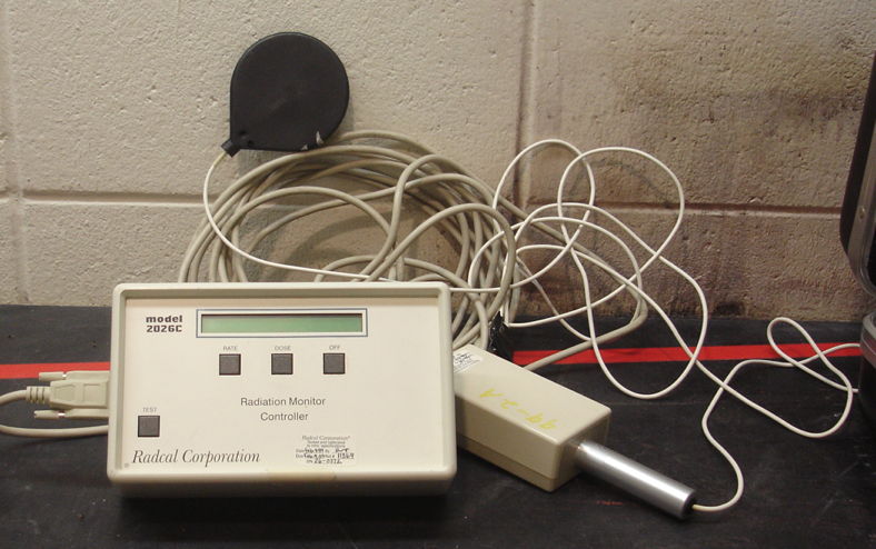
The ionization chamber has volume 60 ml. Its walls are 1.0 mm thick and made of polycarbonate, whose density is 1.2 g/cm3, so the wall density is 0.12 g/cm². The absorption coefficient of polycarbonate we assume is similar to that of polystyrene, so that the chamber will detect most x-rays of energy 7 keV and higher. The disk-chaped chamber is biased with a few hundred volts. No avalanching of electrons takes place within the chamber. The dosimeter measures either the current flowing out of the chamber or the total charge that has flowed out of the chamber, to obtain dose rate or total dose. It is sensitive to dose rates as low as a few μR/s and doses as low as a few μR. The gas in the chamber is air at atmospheric pressure. The chamber is not sealed. It measures the ionization charge in air, and so obtains a direct measurement of the dose in Roentgen (C/kg in air). In response to a short pulse of x-rays, its dose measurement takes roughly four seconds to settle upon its final value.

Eberline PIC-6A

Below we see our second ionizing chamber. It is an Eberline PIC-6A that we believe was manufactured in the 1970s. The ionizing chamber is integrated into the enclosure, with a window on the bottom side as seen in the photograph. This device measures only dose rate, not total dose, but it is sensitive down to 0.3 μR/s. We describe this instrument's performance in detail in our Eberline Report.

Figure: Eberline Dosimeter. The wires emerging from the box allow us to measure dose with automatically.

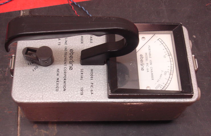
The PIC-6A attains its impressive sensitivity to dose rate by avalanch multiplication of ionization charge. It applies of order 3 kV to its ionization chamber. Instead of measuring the current flowing out of the chamber, it varies the applied voltage so as to maintain a constant current through the chamber. With avalanch multiplication in the ionization chamber, the current is directly proportional to dose rate and increases exponentially with the applied voltage. The meter on the PIC-6A is driven by the applied voltage and graduated logarithmically. Thus the device provides a wide range of operation. With two range settings, it can measure 0.3 μR/s to 0.3 R/s.

Because the PIC-6A measurement requires at least one second to reach equilibrium. Thus the PIC-6A is not able to measure the dose delivered by x-ray pulses. It turns out that many other hand-held ionizing chambers work the same way as our PIC-6A. The new digital-readout device used by the Brandeis University radiation safety office operate the same way, and has a response time of one or two seconds. Neither of these avalanche-based measurements can give us an accurate measurement of the dose delivered by an x-ray pulse.

Image Sensors

Our Image Sensor Dosimeters are sensitive to low dose rates and high dose rates. We can read them out with the LWDAQ easily. The image sensor converts dose into charge in the same way that it converts light into charge. The TC255 is a radiation-hardened image sensor from Texas Instruments, now obsolete. We have plenty of them on hand, so we still use these to measure ionizing dose. Our newer image sensor is the larger ICX424AL. Although not as resistant to radiation as the TC255, the ICX424 has lower dark current when undamaged, and so is better at measuring low dose rates. The KAF-0401E is another image sensor we use both as a dosimeter and as an for taking x-ray images. We have several with phosphor coatings that are far more sensitive to x-rays than bare silicon image sensors. The coated sensor acts like an x-ray film, and provides us with x-ray images of metallic objects illuminated by x-ray pulses.

Pulsed X-Rays

We set up our x-ray source to pulse for 0.5 s every 30 s and measure the average intensity of the image we obtained with a TC255 image sensor. To generate and measure each pulse, we used the Dosimeter Instrument with a 2-s exposure time and a hexadecimal activation command of 3200. We placed the TC255 roughly 50 cm from the source. As we show elsewhere, the charge density in a TC255 dosimeter increases by roughly 523 counts/px/R in response to our pulsed x-rays. Using this constant of proportionality, we converted the charge density in the image sensor into radiation dose.

Figure: X-Ray Pulse Stability. Each point in this graph is the avearge of 50 measurements taken every 30 s. We obtain the dose from the charge density in the TC255P image sensor.

The dose is stable to ±1%. We see a 24-hour variation of ±0.5%. We do not know the source of this variation. With twenty thousand exposures each of 92 mR, the total dose absorbed by the TC255P was 1.8 kR. A dose of 1.8 kR is 16 Gy in air (see above. To determine the dose received by the silicon in the sensor, we must convert Gray in air to Gray in silicon, and for that we need to know the spectrum of our pulsed x-rays.

The graphs below show how aluminum aborbers attenuate the dose received from our pulsed x-ray source. Graphs like these allow us to estimate the spectrum of the x-rays it emits.

Figure: Charge Density for Image Area Pixels with Ionization Chamber Dose versus Aluminum Absorber Thickness. The image sensors and Radcal ionization chamber are 100 cm from the source. The source emits two pulses of 500 ms each for the two image sensors. The ionizing chamber dose is accumulated during 1000 ms.

The table below divides the energy spectrum of our x-rays into intervals. For each interval, we use aluminum absorbers to determine the proportion of the dose carried by photons in the interval. For a description of the procedure by which we measured the spectrum, see here. For each interval we give the average ratio of the silicon and air absorption coefficients for x-rays in the interval. We perform a weighted sum of these ratios and arrive at an average conversion factor between Gray in air to Gray in silicon for our pulsed x-rays of 7.3.

Figure: Spectrum of Our 60-keV Pulsed X-Ray Source, and Average Conversion Factor.

We would like our x-rays to be energetic enough that they are almost certain to penetrate electronic component packages, image sensor windows, and printed circuit boards. A 0.34 g/cm² aluminum plate absorbs almost all x-rays below 14 keV. With such an absorber, our pulsed source will provide 22 mR at range 100 cm once every 30 s, which gives us 44 mR/min, or 440 R/wk, or 39 Gy/wk in air, or 280 Gy/wk in Si.

Continuous X-Rays

[12-DEC-13] Our continuous x-ray source is a K5039S high-stability 50-keV x-ray tube. It has a 0.13-mm beryllium window, whose mass density is therefore 0.024 g/cm². Given the absorption coefficient of beryllium, we expect most x-rays above 2.5 keV to penetrate the window, but very few below. At the start of the day, we take ten minutes to ramp up the power supply of the x-ray tube. Thereafter, we can turn it off as quickly as we like, and ramp it up in one minute. We use the CXRC tool to ramp up the source and monitor its temperature.

The following graph shows the dose rate we observe at position 100 cm on our measuring tape. We believe the source to be somewhere in the range 15-20 cm. The change in the dose with absorber thickness allows us to estimate the spectrum of our continuous x-ray source. The difference between the response of the image sensor dose and ionizing chamber dose for thin absorbers is due to the prevelance of x-rays between 7 keV and 14 keV. These penetrate the ionizing chamber walls but to not penetrate the image sensor window.

Figure: Charge Density for Image Area Pixels with Ionization Chamber Dose Rate versus Aluminum Absorber Thickness. The image sensors and Radcal ionization chamber at location 100 cm on our ruler. We expose the image sensors each for 500 ms. Note that the density of aluminum is 2.7 g/cm³.

With a 0.34 g/cm² aluminum absorber, the x-rays in the remaining dose will be almost entirely above 14 keV. These are sufficiently energetic to penetrate the windows and plastic packages of integrated circuits on the surface of a printed circuit board without significant attenuition. Such x-rays are useful for radiation tolerance tests. The continuous source gives us roughly 0.6 R/min at position 100 cm with a 0.34 g/cm² aluminum absorber, which is 6 kR/wk, or 530 Gy/wk in air, or 3.9 kGy/wk in Si. Almost all this dose will be x-rays above 14 keV. At range 100 cm, we would expect 2.8 kGy/wk, which is ten times the dose rate we obtain with our pulsed source.

[04-APR-14] We place a fresh ICX424 at position 70 cm. We place a 0.34 g/cm² aluminum absorber in front of the source. Our Radcal dosimeter measures 1.70 R/min at the image sensor. Our x-rays should be between 14 keV and 50 keV, for which the absorption coefficient of Si is 7.3 times greater than for air. We multiply 1.70 R/min by 3.84 to convert to Gy/hr in silicon and so obtain 6.5 Gy/hr in Si. We take images with a 50-ms exposure time and 40-ms readout time. The charge density in the images is 0.77 count/px. The sensitivity of the ICX424 is 0.12 count/px per Gy/hr for 14-50 keV x-rays.

[09-SEP-14] We have a 0.34 g/cm² aluminum absorber in front of our source. We move our Radcal ionization chamber along our measuring tape. At each position we turn on the continuous source, measure the dose rate, and turn off the source. We believe the source is somewhere in the range 15-20 cm on the ruler. We try various ranges until our measurements best fit an inverse square law, and so conclude that the effective source position is 18.5 cm. We obtain the following graph of dose rate versus range.

Figure: Dose Rate versus Range for our Continuous X-Ray Source. The slope of the graph is −2.00. To obtain our ruler position, we add 18.5 cm to the range. We have a 0.34 g/cm² aluminum absorber taped over the source aperture.

Today's dose rates are within 5% of our previous measurements with the same absorber performed since December 2013.

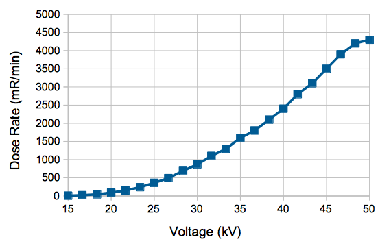
[24-FEB-15] When we turn on the continuous x-ray source, we deliver an increasing control voltage to our 50-kV power supply's current and voltage limit inputs. We increase the voltage and current limits together from 0-1 mA and 0-50 keV. As we do so, the x-ray dose rate at 30 cm range increases as shown below.

Figure: Dose Rate Run-Up at Range 30 cm (Ruler Position 48.5 cm)

[24-JUN-15] Our 50-kV power supply and our two Kevex x-ray tubes are sparking audibly. The 50-kV power supply cannot power a 50-MΩ load. We buy a new 50-keV, 50-W power supply, part number 9700001 from Oxford Instruments. It powers our 50-MΩ load, but our two Kevex x-ray tubes are still sparking, one more than than the other. We buy a new 50-keV, 50-W x-ray tube, part number Jupiter 93000 from Oxford Instruments. This tube does not spark, but it heats up to 40°C after half an hour. We remove the pulsed x-ray source from our lead chamber and open an aperture at the back to allow air to flow through, improving the cooling of the head. The new tube stabilizes at around 32°C. We measure dose rate versus ruler position, and from this deduce that the source is at position 18.3 cm. We convert R/min to Gy/hr with factor 3.8 (Gy/hr)/(R/min) and obtain the following plot.

Figure: Dose Rate (Gy/hr in Si) versus Range (cm from the source) for Kevex and Jupiter sources. We have a 0.34 g/cm² aluminum absorber taped over the source aperture. In September 2015 the Jupiter source is at ruler location 16 cm.

The dose rate for the Kevex and Jupiter sources appears to be the same. At range r, we get 4200/r² R/min = 16/r² kGy/hr in Si, where r is in cm. At range 30 cm, we get 18 Gy/hr.

[30-SEP-15] We have re-built the lead enclosure around our Jupiter source. The fan blows air from the back, so that the air exits through the front opening. We have all-new driver electronics for the x-ray power supply, the door switch, and the wall power relays (Multi-Purpose Device A2081). We have a new x-ray controller script, CXRC V4.2. We calibrate dose versus range with our Radcal dosimeter and obtain the data shown above. The source is now at ruler position 16 cm.

[22-OCT-15] Our continuous x-ray source is once again stable. We combined all control functions on to one circuit, but this did not stop the source from turning off randomly every few hours. In the end, we put a password on the LWDAQ Driver, and that fixed our problem. It appears that some random client connections over the internet were able to shut off the source.

Figure: Flux and Temperature versus Time. The flux is in units of intensity per pixel in a TC255P, and so is a relative measurement. The temperature is on the outside of the case.

We see one halt in x-ray generation, which occurred when at the exact time, to within a minute, that we were monitoring the system remotely. We believe we shut down the source by pressing the wrong button on our control program.

[14-DEC-16] We find that we are running our continuous x-ray source at only 40% of full power. At range 74 cm the dose rate is 1.1 Gy/hr when we expect 2.9 Gy/hr. We increase the voltage to the opto-isolators that drive the x-ray control voltages and obtain 2.9 Gy/hr. We suspect that the opto-isolators have been ageing. The previous calibration of our x-ray flux was SEP-15. We use our CXRC V4.5 script to power up our continuous x-ray source through opto-isolators over 600 s, starting with output voltage and current values of 1.0 and ending at 5.0 at time 600 s. We obtain the following plot of dosimeter charge density versus time.

Figure: Flux versus Time for 600-s Power-Up. The source turns on for output voltages 2.0-3.0 V.

At full power, with range 74 cm (ruler position 90 cm), we measure 770 mR/min with our Radcal dosimeter immediately after power-up, and 750 mR/min after warming up to stable temperature of 30.5°C. We multiply 0.75 R/min by 3.84 (Gy/hr)/(R/min) to get a dose rate in silicon of 2.9 Gy/hr, which agrees with our SEP-15 calibration.

[31-MAY-18] We check the calibration of our continuous x-ray source and rotate the tube so that the x-ray cone is aligned with the red tape on our irradiation table. At range 100 cm we get 1.7 Gy/hr at the cone center and 1.7 Gy/hr at the cone edges. At 50 cm in the center we get 7.1 Gy/hr. We leave the source on over-night. The next morning a temperature measurement of 46.3°C, taking place in the one-minute interval two measurements of 40°C, shuts off the source. We obtain the following plot of temperature and dose rate at range 50 cm.

Figure: Dose Rate and Temperature versus Time. Our dosimeter is a TC255P image sensor at range 50 cm calibrated at 7.1 Gy/hr for charge density 0.95 counts/pixel.

The time constant for warm-up and cool-down is around twenty minutes, reaching equilibrium after an hour. We turn up the fan, raise our shut-off temperature to 50°C, decrease the frequency with which we check the temperature, and try again.

[06-AUG-18] We measure dose rate versus range along the center of our x-ray beam and obtain this plot. We test several absorbers in the beam. Note that we already have a 0.34 g/cm² absorber right on the source, to remove photons below 14 keV.

Figure: X-Ray Absorption by Various Materials.

The absorption coefficient we obtain for lead is ten times lower than predicted above. We have taken no steps to block scattered x-rays from reaching our dosimeter. The coefficients for wood and fiberglass are consistent with those of polyethylene and pyrex respectively.

[06-FEB-20] We have a new set of cables and a new power supply, following chronic sparking in the system. We connect to our X-ray head and power up. We re-calibrate dose rate versus range. The x-ray source is now at ruler position 15.5 cm.

Figure: Dose Rate (Gy/hr in Si) versus Range (cm from the source). We have a 0.34 g/cm² aluminum absorber taped over the source aperture. X-ray source at ruler position 15.5 cm.

[30-OCT-20] We have a new Jupiter 93000 x-ray head from Oxford Instruments. Calibration sheet here. We now have four tubes. Tubes No1 and No2 are K5039S made by Kevex, No3 and No4 are 93000 by Oxford Instruments. No1 draws 3.6 mA at 3 kV, rather than 1 mA at 50 kV. No2 runs for several hours 1 mA at 50 kV before causing a discharge that resets our X-Ray Controller. No3 draws no filament current: the filament is open-circuit. No4 we have yet to test, but we will make sure its filament current is 1.5 A, given a recommended maximum of 1.7 A.

Gamma Rays

[22-APR-14] Brandeis Univeristy has a cesium-137 source powerful enough to perform radiation tolerance experiments. The decay of cesium-137 produces 660-keV gamma rays. At 660 keV, the energy absorption coefficient of air and silicon are almost exactly equal. A dose of 1 Gy in air will produce a dose of 1 Gy in silicon as well. The source enclosure allows us to place our electronics in three posisions. The most uniform dose is at the farthest position, Position 3, which is 20 cm from the source. On 01-JAN-1986, the dose rate was 156 R/min at Position 3 with no lead absorbers. The half-life of cesium-137 is 30.17 years. On 15-APR-14, we expect 82 R/min in Position 3 with no absorbers. This 82 R/min will deposit 0.72 Gy/min in air. Because the energy absorption coefficient of silicon and air are both 0.030 cm²/g for 660-keV gammas, the dose will also be 0.72 Gy/min in silicon, or 43 Gy/hr in Si.

Figure: Lead Absorbers for the Cesium-137 Irradiation Chamber. The dime is 17.9 mm in diameter, so the lead is 22.0 mm thick.

We install two lead absorbers that come with the ¹³⁷Cs irradiation chamber, which the manufacturer states will give us dose attenuition of ×10 within the chamber. By interpolating NIST scattering coefficient measurements for photons in lead, we get 1.0 g/cm² at 660 keV. A 2.2-cm thick lead absorber will transmit roughly 1−exp(−2.2/1.0) = 89% of photons, which is close to the ×10 attenuition. With these in place, our calculated dose rate at Position 3 is 4.3 Gy/hr.

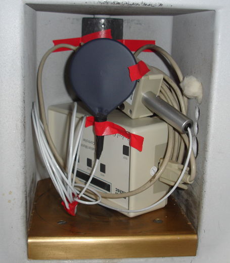
We put our Radcal dosimeter inside the radiation chamber, as shown below. We locate the Radcal's ionization chamber at mid-height above Position 3. We close the chamber and raise the source for a total of 3.05 minutes, during which we accumulate 17.5 R. Our measured dose rate at Position 3 is 5.7 R/min or 3.0 Gy/hr.

Figure: Radcal Dosimeter in Cs-137 Irradiation Chamber. The Radcal's 60-cc ionization chamber is the black disk. Note the lead absorbers in the background. Dose rate with the source raised is 5.7 R/min or 3.0 Gy/hr.

We place an ICX424 at Position 3 and obtain the following image. The average intensity is 28 counts, maximum is 116 counts, well below the saturation level of the sensor.

Figure: Cesium-137 Gamma Rays in ICX424 Image Sensor. Image displayed with exact intensification. Calculated dose rate is 4.3 Gy/hr, measured dose rate is 3.0 Gy/hr. Image area exposure time is 50 ms, charge density 0.22 count/px.

Our Radcal dosimeter was re-calibrated in September 2013. The Cs-137 irradiation chamber was calibrated by the manufacturer in 1986. We have used our Radcal dosimeter in all our x-ray experiments and calibrations of image sensor dosimeters, so we will use its measurement of Cs-137 dose for our experiments, knowing that the actual dose in received by our electronics might be greater than that measured by the Radcal, but unlikely less. Thus at Position 3 with the ×10 absorbers, we get 3.0 Gy/hr.

[13-JAN-17] We repeat our calibration of our Cs-137 source. We place the ionizing chamber at Position 3, 20 cm from the source, as shown here. We accumulate 13.6 R in 3 minutes, which is 4.5 R/min compared to 5.7 R/min in April 2014. The dose rate at Position 3 appears to be close to 2.4 Gy/hr in Si. The calculated dose rate for Position 3, using the original Cs-137 calibration, is 4.0 Gy/hr (down from 4.3 Gy/hr three years ago).

Neutrons

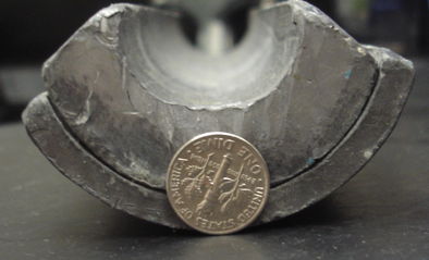
[13-JUN-18] Our californium-252 (Cf-252) source produces neutrons with maximum kinetic energy 13 MeV, energy is 2.3 MeV, and most probable energy 1 MeV. The half-life of Cf-252 is 2.6 years. The source activity today is 2.4 μCi × 37 GBq/Ci = 89 kBq. Of these 89k decays per second, 3.1%, or 2.7k, are spontaneous fission, producing 2,700 neutrons per second. The maximum energy of the neutrons is 13 MeV, the average energy is 2.3 MeV, and the most probable energy is 1 MeV.

Figure: The Californium-252 Capsule. Dimensions in inches. Outer diameter of cylinder is 9.4 mm.

The source is enclosed in a stainless steel cylinder as shown above. For more drawings and activity calculations see Cf252_Data. When we place our radiation target at the end of the cylinder, the neutrons must first travel through 15 mm of steel. The likelyhood of a neutron interacting with an iron nuclus is given by its cross-section, which depends upon energy as shown below.

Figure: Total Interaction Cross Section for Neutrons in Iron-56. Units are barn.

We use the cross-section to estimate the attenuition of neutron flux with distance. The probability of a neutron passing through a thickness x of a material is given by exp(−xαd), where α is the cross-section and d is the number of atoms per unit volume. If we imagine that each atom occupies a cubic volume, and view the cross-section as the effective area for interaction presented to the neutron by the atom within its volume, we can arrive at the above equation as follows.

Figure: Penetration of Particles with Known Cross Section through a Material.

Of the neutrons passing along the axis of the cylinder, 60% will reach the end of the cylinder without interacting, while 40% will be scattered in all directions before they reach the end. Of the neutrons that travel out from the source along the 4.7-mm cylinder radius, 85% will escape the cylinder and only 15% will scatter in the steel. The neutron flux emerging from the end of the cylinder will be dominated by neutrons that come straight from the source without interacting. The direct neutron flux per square millimeter at the end of the cylinder will be roughly 2.7k × 0.60 / (4π × 15 × 15) = 0.58 n/s/mm2 = 58 n/s/cm2. But the scattered neutrons will most likely emerge from the steel as well, so we estimate that the flux at the end of the cylinder will be closer to 2.7k × 1.00 / (4π × 15 × 15) = 0.95 n/s/mm2 ≈ 100 n/s/cm2. Given that neutrons in the range 0.5-10 MeV have roughly the same 1 MeV-eq. KERMA (see here), the neutron dose rate is roughly 100 1-MeV eq n/cm2/s, or 6.0 × 10⁷ 1-MeV eq n/cm2/week. It will take three hundred years to accumulate 1 Tn. At the inner radius of the nSW in ATLAS, we expect to accumulate 1 Tn per year. We use this source to study fast neutron damage to image sensors. The dose rate may be low, but we have eighty thousand pixels per image sensor, so we observe bright pixels appearing over days and weeks.

Expected Doses

[27-APR-16] The Brandeis University High Energy Physics Electronics Shop makes alignment devices for high energy physics experiments. We installed thousands of BCAM and RASNIK devices in the ATLAS end-cap muon spectrometer. The radiation doses received by these devices depends upon their location and is proportional to the integrated luminosity accumulated by the ATLAS detector. During its first decade, 2007-2017, LHC will operate at peak luminosity 1×10³⁴ 1/cm²s and accumulate integrated luminosity 300 1/fb. During its second decade, 2020-2030, LHC will operate at peak luminosity 5×10³⁴ 1/cm²s and accumulate 3000 1/fb. The muon drift tube (MDT) chambers of the end-cap muon spectrometer are arranged in four vertical disks named EIMDT, EEMDT, EMMDT, and EOMDT. The EIMDT disk is the closest to the interaction point, and receives the largest dose of both ionizing and neutron radiation. This disk will be replaced after 300 1/fb with the New Small Wheel (nSW). The nSW will endure the radiation generated by 3000 1/fb. The other MDT disks must endure the radiation generated by 3300 1/fb, because they will remain in the ATLAS dectector through both decades of its operation. Because these other disks are farther from the interaction point, however, the doses they receive will be less. In this section, we consider how much radiation we expect our devices to receive, and what form it will take. For the results of our radiation tolerance tests, see Irradiation Tests.

Almost all proton-proton interactions at the center of the ATLAS detector result in two protons moving off at a slight angle to the original beam direction. These protons collide with the beam pipe several meters from the interaction point, and produce a shower of radiation. This radiation emerges through the shielding around the beam pipe and enters the detector. The intensity of the radiation in the ATLAS end-cap decreases with radius from the beam line, as well as with distance from the interaction point. The following plot shows the simulated total ionizing dose in the ATLAS detector using the 2012 geometry. We obtained the plot as a ROOT file from this archive of simulation results.

Figure: Simulated Total Annual Ionizing Dose for Annual Integrated Luminosity 100 1/fb. The simulation assumes collision energy 14 TeV (7 TeV per beam) and the 2012 detector geometry. Point (0, 0) is the interaction point. The archive does not specify if the dose is in air or silicon. The horizontal axis is z and the vertical axis is r. For a plot of photon flux in kHz/cm² at luminosity 10³⁴ 1/cm²s see here.

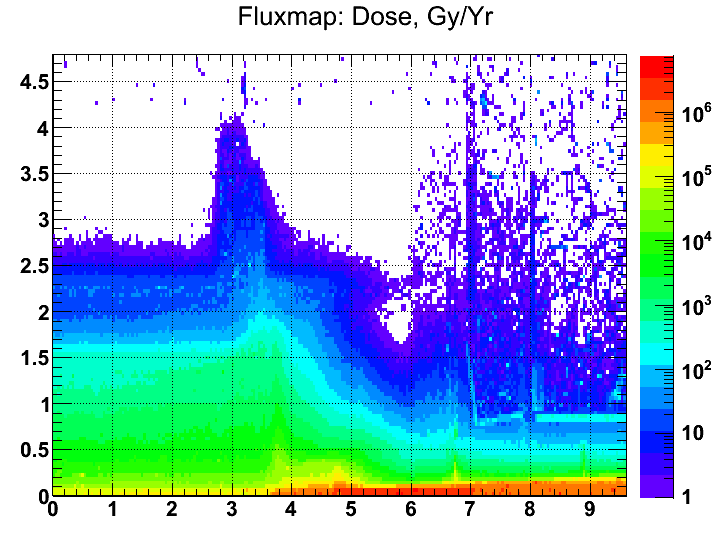
Because this radiation tells us nothing about any particular collision between protons, and yet causes hits in the end-cap muon detectors,it is called the ATLAS background. The moun detectors must be able to accommodate the background hit rate and still detect the muons traveling from the interaction point. The following plot shows the simulated 1-MeV equivalent neutron dose in silicon in units of kHz/cm² at luminosity 10³⁴ 1/cm²s. To obtain the dose for 100 1/fb we multiply by 10⁷ s effective run-time.

Figure: Simulated Silicon 1-MeV Equivalent Neutron Flux at Luminosity 10³⁴ 1/cm²s. The simulation assumes collision energy 14 TeV and 2012 detector geometry. Point (0, 0) is the interaction point. The horizontal axis is z and the vertical axis is r.

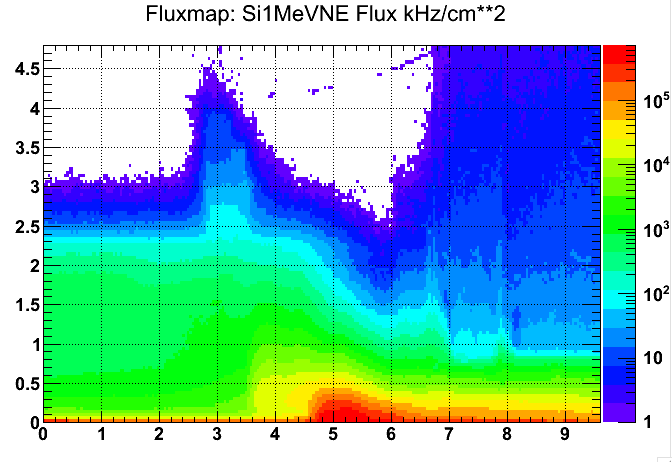
We note that we do not know if the simulation is measuring the dose in aluminum, argon, air, or silicon. Nor does the simulation give us any clue as to the distribution of photon or neutron energy. Furthermore, the resolution of the map is poor in most of our MDT regions. In order to be certain that we have the doses in silicon, rather than aluminum or air, we calculated our own doses from particle lists, as we describe below. We begin with calculations in EIMDT and move on the EMMDT.

In the ATLAS note "A FLUGG-based Cavern Background Simulation Application", Bougher et al. describe how they simulate the background radiation environment in the ATLAS detector. We obtain from the ATLAS Background Radiation group a 1-GByte text file of 3.7 million lines, archived in ATLAS_All_R0.zip. Each line describes a simulated radiation particle or photon entering one of two dozen scoring volumes in the ATLAS detector. From now on, we will use "particle" to refer to any product of radiation, particle or not. The list is the result of ten thousand simulated proton-proton interactions with total cross-section 72 mbarn at collision energy 14 TeV. The scoring volumes numbers are described in region.c. The particle codes are listed on the FLUKA website. We extract all particles that enter the MDT scoring volumes using a Toolmaker script, archived in Scripts.tcl. Each line in the new list is a particle as in the original list, but we omit some parameters, convert the units of other parameters, and add the radius from the beam line on the end of the line. Our own particle line format we calle "R1", while the format in the original FLUGG file is "R0". Our list of all particles entering the MDT volumes is MTD_All.txt.

Scoring Volumes 5 and 6 contain the EIMDT disks of the two end-caps. Volume 6 spans r = 0.82-4.54 m and z = 7.05-7.90 m. Within this disk, we have devices at a minimum radius 2.2 m. For the purpose of estimating the dose received by the alignment devices at this radius, we define a volume extending from r = 2.1-2.3 m and from abs(z) = 7.05-7.90 m. We call this Volume X. We note that Volume X has two parts, one in each end-cap.

We want a list of particles entering Volume X. We start by extracing from MTD_All.txt a list of all particles entering Volumes 5 and 6, which we call MDT_EI.txt. We extrapolate the trajectory of each of these particles and determine if it intersects Volume X. If so, we add it to a list of particles we assume will enter Volume X, which we call MDT_EI_X.txt. We append to the information on each particle the length of its track through Volume X, which is essential for the calculation of deposited energy. Our code for performing extrapolation and intersection to generate the new list is Intersect.pas. We assume these particles do not interact with the material within the EIMDT volume outside Volume X. This assumption is justified if most particles are entering Volumes 5 and 6 through Volume X, which proves to be the case. The assumption is justified if most particles are of sufficiently high energy that their probability of interaction outside Volume X is low, which also proves to be the case. Our assumption allows us to use our list of particles that intersect Volume X as our list of particles that actually pass through Volume X. Our assumption allows us to ignore any loss of particles due to interactions outside Volume X, and is allows us to ignore the products of such interactions outside Volume X.

We start with a list of 3.7E6 particles entering all the ATLAS scoring volumes. Of these, we extract 1.4E6 that enter the MDT volumes. Of these, 7.6E5 enter the EI volumes. Of these 2.5E5 intersect Volume X. Thus we obtain a list of particles we can use to represent the radiation entering Volume X in ten thousand proton-proton interactions at 14 TeV.

The dose is dominated by photons and neutrons. We use a script to extract all the photons into one file MTD_EI_X_Photons.txt and all the neutrons into another file MTD_EI_X_Neutrons.txt. We use a script to make a histogram of the photon and neutron energy, which allows us to make the following plots of the energy spectra of neutrons and photons. Almost all photons are in the range 0.1-10 MeV, for which the energy absorption coefficient of all materials is the same to within ±20%. For such photons, a calculation of ionizing energy deposited per kilogram of air (Gy in air) will apply well to aluminum (Gy in Al) and silicon (Gy in Si). The map above does not specify a material, but we see that the energy of the photons is such that, the material makes little difference to the dose, provided the material is something like air, silicon, or aluminum, and not lead.

Figure: Simulated Spectra of Photons and Neutrons at Inner Edge of EIMDT. Quantity is the number of particles of each energy entering our Volume X as a result of ten thousand 14-TeV proton-proton interactions. The bin for <=1keV neutrons contains roughly 40,000 thermal neutrons.

The peak in the photon spectrum at 500 keV corresponds to positron annihilation. The peak at 8 MeV corresponds to prompt gamma emission after the capture of thermal neutrons by iron. This prompt gamma peak accounts for most of the ionizing dose. If there were no photons above 10 MeV, we would assert that some kind of binning cut-off has occured in the simulation. But there are a few dozen photons above 10 MeV, although not enough to be visible in the plot above.

To calculate the ionizing dose in Volume X, we determine for every photon the length of its path through Volume X. We make a histogram of total path length versus energy. We divide the total path length in each energy bin by the volume of Volume X, and so obtain the path length per unit volume for photons of each energy. We multiply by the path length per unit volume by the absorption coefficient of silicon. We divide by the density of silicon, 2.33 g/cm³, and multiply by the bin energy itself to obtain the energy deposited by photons in this bin per unit mass of silicon during ten thousand proton-proton interactions. We multiply by the proton-proton cross section, 72 mbarn, and by the integrated luminosity we hope to attain by the end of ten years at higher luminosity, which is 3000 1/fb, and so obtain the total expected dose from each energy bin. When we add these doses together, we obtain a total dose of 85 Gy in Volume X. For 100 1/fb, we obtain a dose of 2.8 Gy in Volume X, while the map above suggests a dose closer to 2.2 Gy.

Figure: Simulated Doses of Photons and Neutrons at Inner Edge of EIMDT after 3000 1/fb, Plotted versus Photon and Neutron Energy. The units of photon dose are Gray in Si, and of neutron dose are Tn, which is 10¹² 1-MeV eq. n/cm².

For each neutron entering Volume X, we calculate the length of its path through Volume X. We make a histogram of total path length versus energy. We divide the total path length in each bin by the volume of Volume X, and so obtain the path length per unit volume for neutrons in each bin. We multiply by the path length per unit volume by the 1-MeV eqivalent displacement KERMA of each energy, and so obtain the average 1-MeV eq.n/cm² dose at each energy for the entire volume. We scale this dose for total integrated luminosity and cross section, and so obtain the 1-MeV eq.n/cm² dose delivered by the neutrons in each bin. When we add all the bins together, we obtain a total dose of 6.4 × 10¹² 1-MeV eq. n/cm² = 6.4 Tn for 3000 1/fb. For 100 1/fb, we obtain a dose of 0.21 Tn in Volume X, while the map above suggests a dose closer to 0.15 Tn.

We use Intersection.pas and our Toolmaker scripts to calculate the simulated ionizing and neutron dose in EIMDT with increasing radius. At each radius, we create an annulus from r−10% to r+10% and use the average dose in this volume as our simulated dose. If all goes well, the LHC should deliver a total integrated luminosity of 3000 1/fb. The instantaneous luminosity after the upgrade may reach as high as 7×10³⁴ 1/cm²s. If we combine this luminosity with 10⁷ s/yr and 10 year of operation, we arrive at 7000 1/fb. But the beam average luminosity will be much lower, resulting in a target of 3000 1/fb. We plan to install electronics in the New Small Wheel (nSW) during the Phase I upgrade. At that time, LHC should have delivered 100 1/fb already. But we will assume that the nSW must endure the dose generated by the entire 3000 1/fb. The plot below shows the total simulated dose we expect after 3000 1/fb at 14 TeV in the nSW as a function of radius from the beam line.

Figure: Simulated Total Ionizing and Neutron Dose in EI Layer versus Radius for Integrated Luminosity 3000 1/fb and Collision Energy 14 TeV.

We plan to place cameras at a minimum radius of 2.2 m. Our calculations suggest the dose at 2.2 m will be 85 Gy and 6.4 Tn. The radiation maps supplied by the ATLAS Background group suggest doses of 66 Gy and 4.5 Tn. The spreadsheets supplied by the CERN radiation tolerance group specify doses of 57 Gy and 4.7 Tn.

We now consider the dose at the inner edge of EMMDT. The EM scoring volumes span z = 13.65-14.54 m and r = 1.74-11.82 m. These values agree well with our own MDT drawings. Our alignment devices are at a minimum radius 1.92 m. We begin by extracting all EM particles from our simulation list. We define Volume Y as z = 13.6-14.6 m and r = 1.90-2.10 m. We use use Intersection.pas and our Toolmaker scripts to obtain a list of particles passing through Volume Y.

We calculate the dose at a selection of radii in EM for 3000 1/fb and so produce a plot of simulated dose versus radius in EM.

Figure: Simulated Total Ionizing and Neutron Dose in EMMDT Layer versus Radius for Integrated Luminosity 3000 1/fb and Collision Energy 14 TeV.

At 1.9 m, in Volume Y, the dose is 16 Gy and 0.4 Tn. According to the CERN Radiation Tolerance group's spreadsheets, the dose at this radius in EMMDT is 79 Gy and 0.18 Tn. We know that their spreadsheet does not account for the additional shielding inside EMMDT that was added to the ATLAS geometry in 2003, so we expect their ionizing dose to be too high.

[08-JAN-14] We investigate the peak in the photon spectrum at 8 MeV. We make a list of all photons 7-10 MeV and plot a histogram of their arrival time in Volume X, in seconds after the simulated interaction.

Figure: Arrival Time of Simulated 7-10 MeV Photons. We examine Volume X.

Volume X is roughly 7 m from the interaction point, or 23 ns at the speed of light. We see the first photons arriving at around 23 ns. We have a prominent peak at 1 μs. We plot the frequency in 1-μs bins here, and observe that the plot looks like a nuclear decay with half-life 1 μs. Our best guess is that neutrons in the simulation are activating the brass shielding material, resulting in a simulated gamma-decay with half-life 1 μs that releases one or more 8-MeV gammas.

[26-JUN-15] During consultation with collaborators at CERN, we learn that the 8-MeV gammas in our simulation are produced by the capture of thermal neutrons by Fe-56. The Fe-56 becomes Fe-57, which relaxes with the emission of photons between 5.9 and 7.6 MeV, as discussed in Fiebiger et al.. These gammas are "prompt gammas", which means they are emitted immediately the thermal neutron is absorbed. Thermal neutrons travel at 2000 m/s. There is plenty of iron in the JD shielding component of the ATLAS detector, near Volume X. The shielding is of order one meter thick. Thus thermal neutrons generated by a collision will remain in the JD for of order microseconds, and appear after a fraction of a microsecond, which is consistent with our arrival time plot above. And so we conclude that the Volume X ionizing dose is dominated by prompt gammas emitted by iron of the JD shield. These 5-8 MeV gammas have the same absorption coefficient in aluminium, air, and silicon, so whether the material in the ATLAS background simulation is air or aluminum in a particular place, we can use the dose for silicon as well.

Observed Doses

[08-JAN-13] We have an entire set of ATLAS end-cap alignment system images from Christoph Amelung. They are dated FEB-13 and all are TC255 images. We are looking for signs of neutron damage, as we describe in this report. For each 10¹² 1-MeV eq. n/cm² neutron dose, the TC255 dark current increases by 0.28 counts/ms at 20°C. As we describe elsewhere, the TC255s that receive the highest neutron dose are in our Volume X, around z = 7.5 m, r = 2.2 m. These receive 1 MeV eq. n/cm² flux of 10 kHz for luminosity 10³⁴ cm²/s and 14 TeV collision energy. This graph shows roughly 22 1/fb at 7 TeV recorded in ATLAS so far, leading up to the February 2013 shut-down.

To the first approximation, integrated luminosity 22 1/fb at 7 TeV generates the same amount of radiation as 11 1/fb at 14 TeV. According to our calculations, objects in Volume X have received roughly 0.011 Tn, so the TC255 dark current should be 0.0042 counts/ms. We read out each row of the TC255 in 172 μs, so 0.004 counts/ms would appear as 0.0006 counts/row. Our resolution in measuring dark current is 0.0007 counts/row, so we will need a large number of images to notice the damage. We analyzed all FEB-13 images from the end-cap. There are 10 images with dark current above 0.005 counts/row, and these all have something wrong with them. The rest go from 0.005 down to −0.001 counts/row. We sort them all by name and go through the list, but the sensors in Volume X do not have higher dark current than those elsewhere.

[05-AUG-14] We receive the following image from the ATLAS end-cap CSC alignment system, at r = 2.0 m and z = 7.5 m. This particular source is dim, for some unknown reason, and requires a flash time of 100 ms compared to the usual 1 ms.

Figure: TC255 Image from CSC Alignment Camera, a 100-ms Exposure with Exact Intensification. We see three bright spots from neutron damage along with the the larger light source image.

We obtain a background-subtracted image from the same camera, and the three bright spots disappear, while the light source image remains.

Figure: Background-Subtracted TC255 Image from CSC Alignment Camera, a 100-ms Exposure with Exact Intensification. Vertical smearing of the spot is a feature of the pin-hole camera optics.

These bright spots are pixels damaged by fast neutrons. These pixels generate dark current. The longer the exposure time, the brighter they become.

[28-APR-16] We receive five freshly-captured images from a CSC camera in ATLAS, at roughly z = 7.5 m and r = 2.0 m. The bright pixels in the images have been damaged by neutrons. We read the images into our Dosimeter Instrument. We set the threshold "1 $", which will find all pixels more than one count above the average intensity, add their above-threshold intensities together, and divide by the number of pixels in the analysis bounds to obtain the damage intensity in counts/pixel. We divide by the exposure time to obtain dark current in counts/ms.

The camera is at z = 7.5 m and r = 2.0 m. According to this NIEL map, we expect the image sensor to receive a 0.20-Tn neutron dose per 100 1/fb at 14 TeV. At the time we obtained this image, LHC had delivered 5.6 1/fb at 7 TeV (3.5 TeV per beam) in 2011, 23 1/fb at 8 TeV in 2012, and 4.2 1/fb at 13 TeV 2015, which is equivalent to 20 1/fb at 14 TeV, which is 20% of the luminosity at which our image sensor would receive 0.20 Tn. So this sensor has endured 0.05 Tn. Thus we can calculate, for each image, the apparent neutron damage rate in counts/ms/Tn. According to our model of neutron damage, we expect 0.28 counts/ms/Tn at 20°C, or 0.014 counts/ms after 0.05 Tn.

Our best measurement of the neutron-damage dark current is from the 100-ms dark exposure. We see 0.0014 counts/ms, which is ten times smaller than our model predicts. It could be that damage caused by the ATLAS neutron spectrum anneals at room temperature more quickly than the damage caused by our neutron irriadiation test spectrum. The ATLAS spectrum has more 100-keV neutrons than our irradiation tests. Whatever the explanation, the fact remains that 20 1/fb causes 0.0014 counts/ms of dark current in the TC255P at the innermost radius of EIMDT. After 300 1/fb we expect the dark current to reach 0.021 counts/ms. A 100-ms exposure will then result in only 2.1 counts/pixel of dark current. We can tolerate 100 counts/pixel and still maintain BCAM precision.

[06-MAY-16] We obtain 96 images from the CSC alignment system of the ATLAS end-cap, each with no light source flashing, 100 ms exposure, and each image saved as a file with the name of its image in the ATLAS data acquisition database. We reject one image because it contains nothing but noise, and use the remaining 95.

Figure: Charge Density in CSC Images. The columns are charge density in counts per pixel, slope of intensity in counts per row, average intensity (background intensity) in counts, threshold intensity for spot-finding in counts, and then the net intensity of the brightest spot in the image, for spots with at least one, two, three, and four pixels.

The spot with the greatest net intensity contains three pixels that share its net intensity of 158 counts. No spots are so bright that they saturate the image sensor in these 100-ms exposures. The average charge density is 0.095 counts/pixel, which implies dark current of 0.00095 counts/px/ms. Assuming integrated luminosity of 20 1/fb, the ATLAS background simulation suggests a dose of 0.05 Tn for these sensors. The dark current generation by the neutron dose appears to be 0.019 counts/ms/px/Tn.

[11-JAN-19] The plot below shows the Run 2 total integrated luminosity in ATLAS.

Figure: LHC Integrated Luminosity for 2015-2018.

We scale the luminosity from 2011, and 2012 with beam energy to get around 15 1/fb. We add to the above accumulation of 140 1/fb and get 155 1/fb at the end of 2018. Going back to Jun 2017 we have 55 1/fb. From that time we have 95 image from r = 2.0 m and z = ±7.5 m with 100 ms exposure and no light sources. The simulated neutron dose delivered to these image sensors is 55 × 8 Tn / 3000 = 0.15 Tn. We measure the dark current in these images in two ways. First we measure charge density in pixels more than two counts above threshold. We get average charge density 0.204 cnt/px with standard deviation 0.06 cnt/px. This is 0.0020 cnt/px/ms = 2.0 mcnt/px/ms, or 13 mcnt/px/Tn. Second, we measure the slope of intensity in the image, which is the dark current accumulating in all pixels as they are read out. The slope is 2.3 mcnt/row ±0.7 mcnt/row. We multiply by the readout speed 5.0 row/ms to get 11 mcnt/px/ms, or 73 mcnt/px/Tn. We do the same calculations for images 19-MAY-2016 and get 19 mcnt/ms/Tn and 90 mcnt/ms/Tn for charge density and intensity slope. We look at image from the EO layer, where the neutron dose is a hundred times smaller, and the charge density and slope of intensity are not significantly different from zero.

[23-MAY-19] We present Neutron Damage of CCDs in ATLAS Endcap at CERN. A few days later, we find that the latest GEANT4 simulation of neutron dose in the EO layer is in better agreement with our CCD dose measurement, see here. We divide the end-cap into many annular regions. In each region, the neutron dose is approximately constant. The average neutron damage rate within each annulus is the average dark current in the image sensors, adjusted for temperature, and divided by the simulated dose in that same region. Each region gives us a measurement of damage rate. The plot below is a histogram of these measurements for the FLUGG and GAENT4 calculations of dose rate.

Figure: Histogram of Neutron Damage Rates for a Set of End-Cap Regions, Assuming FLUGG and GAENT4 Doses. Each measurement of damage rate we make in an annular region where the dose is almost constant.

The damage rate is around 0.12 cnt/ms/Tn, which agrees well with the damage rate we see in the TC255P twenty years after irradiation in Prospoero.

Our image sensors are now acting as neutron dosimeters checking the relative neutron dose in the ATLAS end cap.