Photomultiplier Circuits (A2088)

Contents

Description

We use assembly number A2088 for a family of amplifiers, shapers, high-voltage filters and photomultiplier (PMT) mounting circuits.

We describe each letter version below. We present our initial work on using Silicon Photomultipliers (SiPMs) in Heller et al.. The SiPMs we are working with come from a family made by On Semiconductor, the MICROFC series. In Constructing a Muon Telescope with SiPMs we show how our amplifiers and SiPM circuits can be used, in combination with an oscilloscope and two squares of scintillator plastic, to make a muon telescope.

Amplifier-Shaper, Version One

[13-FEB-19] The A2088A is our first amplifier-shaper. Printed circuit board files in A208801B. The A208801A we aborted because we omitted C7 and C8.

We load two ERA-1SM into the circuit as shown. We measure gain versus frequency for various input powers.

Figure: Gain of A2088A with 2 of ERA-1SM, 3-dB Attenuator, and Increasing Input Amplitude. Plots are labelled in mVpp input amplitude.

We expect the gain to be +12 dBm for each amplifier, −3 dB for the attenuator, is +21 dB. We see up to 19 dB. The amplifier does not produce the +12 dBm output power we expect. We apply a 50-mVpp, 200 kHz input and observe the following output.

Figure: Output of Unmodified A2088A for 50-mVpp 200 kHz input. For 100-mVpp 40 kHz input see here.

For inputs greater than 20 mVpp the amplifier oscillates and its gain at the signal frequency is compromised. Our maximum output amplitude is around 300 mVpp when we expect 3 Vpp.

The shaper we configure after consulting our treatise on pulse shapers. We set L1 = 3.3 μH and C3 = 1 nF. We find that the 100-nF capacitors cause the output baseline to shift. When combined with a 50-&Ohm; signal impedance, thes capacitors introduce a 5-μs time constant. During a 100-ns pulse, we expect the baseline voltage to move up by 2% of the pulse height. We observe something closer to 10%. We place 1-μF capacitors in parallel with the 100-nF coupling capacitors and get the following pulse.

Figure: 40-mV 12-ns Pulse Shaped and Amplified. We have 1-μF coupling capacitors to minimize baseline shift.

[14-MAR-19] We work on the A2088A until it stops oscillating. We have 100-pF coupling capacitors, and for decoupling the power supply we have 100 pF, 100 nF and 1 μF capacitors scattered about. We have top-side ground planes made of copper tape. We have U1 as ERA-3SM and U2 as ERA-1SM, the attenuator is −3 dB, and L1 = 0 H, while C3 is omitted.

Figure=: The A2088A Modified Until It Stops Oscillating.

We apply 100 MHz input and obtain the following plot of output power and gain versus input power in dBm (decibels above 1 mW into 50 Ω).

Figure: Gain and Output Power verus Input Power for A2088A at 100 MHz After Modification.

Each of our four 100-pF coupling capacitors have impedance 15 Ω at 100 MHz, so each of them introduces a loss of 0.4 dB. The ERA-3SM and ERA-1SM should provide gain of around 34 dB. Our attenuator is −3 dB. We expect a total gain of around 29 dB. We observe 23 dB. We expect a maximum output of +12 dBm and that's what we see: 2.2 Vpp into our 50-Ω oscilloscope input.

We add 1-μF capacitors in parallel with all four 100-pF coupling capacitors, and two 10-μF capacitors in parallel with our existing decouplers. At 100 MHz with 70 mVpp input, our output is 1.9 Vpp for gain 29 dB. We measure gain versus frequency.

Figure: Gain versus Frequency for −20 dBm Input. Modified A2088A with ERA-3SM, 3-dB Attenuator, ERA-1SM, 100 pF and 1 μF couplers.

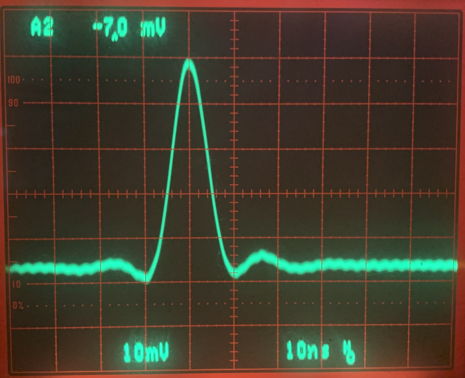
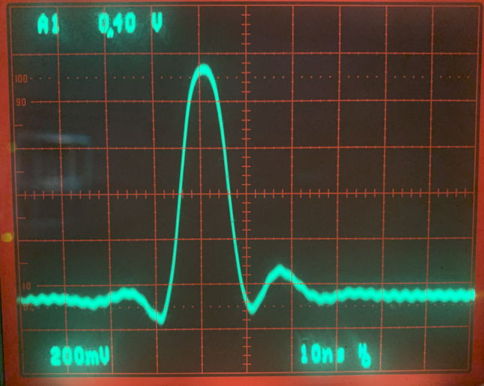
We load 3.3 μH for L1 and 1.0 nF for C3 to make our shaper. We obtain the following for a 200-mV input pulse.

Figure: 200-mV 12-ns Pulse (Top) and Shaped Output (Bottom). Output pulse is 600 mVpp.

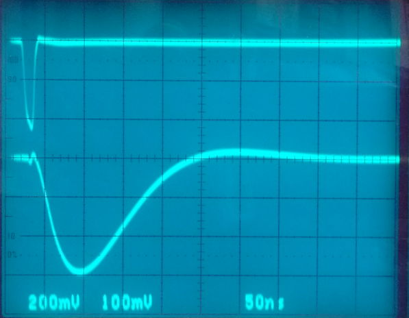
The exact shape of the output pulse, and the amplitude of the small pre-pulse spike, depend upon the arrangement of our coaxial cables near the oscilloscope.

High-Voltage Low-Pass Filter

[01-FEB-19] The A2088B is a low-pass filter for a PMT high-voltage power supply. The high-voltage input, up to 3 kV, is low-pass filtered to remove noise, with corner frequency 4 kHz. SHV plugs receive and transmit the high-voltage power. The 10-kΩ series resistor will drop the high-voltage output by 10 V per 1 mA.

A side port with BNC socket provides a high-pass filtered view of the output high-voltage, with corner frequency 400 Hz. The filter proves effective in removing 100-kHz pulses from the high-voltage, and reducing PMT output noise by around 80%.

SiPM Head, Version One

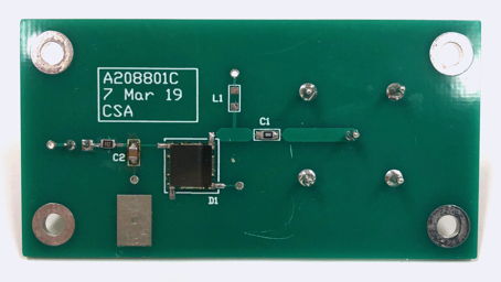
[11-FEB-19] Our silicon photomultiplier (SiPM) Head provides a 6 mm × 6 mm area, 35-μm pixel MICROFC-60035 photomultiplier along with bias and output coupling.

The A2088C-0 is a breadboard version shown below.

Figure: SiPM Breadboard Circuit. Pins 1, 2, and 3 on the SiPM are marked. We deliver 0V and bias voltage VC through wires. The fast output is on an unused pin. By connecting 0V to the input of a current meter, we measure dark current.

We use A2088C-0 to measure dark current versus bias voltage.

Figure: MICROFC-60035 Dark Current versus Bias Voltage at Room Temperature.

The A2088C-1 uses the A208801C printed circuit board. We have L1 omitted, C2 replaced with 1-Ω resistor, and R1 is 1 kΩ.

Figure: The A2088C-1 Made with A208801C PCB. Top (left) and Bottom (right).

[09-DEC-19] We use the A2088C built on A208801C circuit board to detect light pulses emitted by an LED [Need part number, size, wavelength] driven by 12-ns pulses from a function generator. We amplify and shape the pulses emerging from the SiPM with an A2088D-100 (100-ns pulse duration and gain ×40).

Figure: Height of Shaped SiPM Pulse versus Peak Voltage of LED Drive Pulse, for Various SiPM bias voltages.

[11-DEC-19] Suppose photons arrive at the top surface of the avalanche region of our SiPM, as yet unabsorbed, and now have some chance of being absorbed for each incremental distance they penetrate into the avalanche region. Let us assume the electric field is uniform through the thickness of the avalanche region, and assume a maximum avalanche gain of one million. We will get single-photon pulses all of the same height only if all photons are absorbed in the first infinitesimal layer of the avalanche region. But there will be some absorption depth for photons in the silicon, and photons absorbed deeper into the silicon will generate a smaller avalanche, and therefore a smaller pulse. We perform a Monte-Carlo simulation of this process using a Toolmaker script.

Figure: Penetration and Pulse Height for Photons. Photon absorption length is 1% of thickness, maximum avalanche gain is 10⁶. The penetration is a fraction of the thickness of the avalanche region. The height is the fraction of the pulse generated by a photon being absorbed at the surface of the avalanche region.

For the same plot made for 2% absorption length see Sim_1_2 and for 5% absorption length see Sim_1_5. The spread of pulse heights increases as the photons penetrate further. If we increase the gain to 10⁷ the graph looks much the same.

Figure: Penetration and Pulse Height for Photons. Absorption depth is 1% of thickness, maximum avalanche gain is 10⁷.

Let us assume that thermal electrons are generated at random in the avalanche layer, with uniform distribution. We write a Monte-Carlo simulation of this process using another script and obtain the following plot of the thermal pulse rate distribution with respect to pulse height for three different values of maximum gain. We make our histogram with logarithmic bins so we can plot pulse height on a log scale.

Figure: Distribution of Thermal Electron Pulses (Dark Current Pulses). We plot the normalized rate versus the normalized pulse height. This plot for avalanche gain 1 million. The maximum pulse height is the same as that of a photon being absorbed at the surface of the avalanche layer.

The number of pulses in each decade of pulse height is the same, which is consistent with each decade corresponding to its own layer in the avalanche region, and all layers being of the same thickness.

Amplifier-Shaper, Version Two

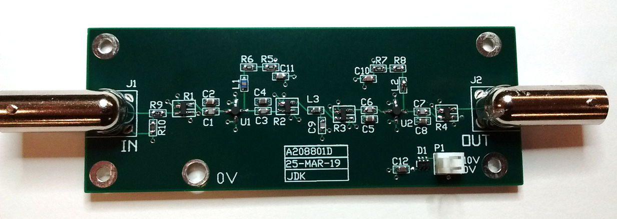
[20-MAR-19] Our second amplifier-shaper has four copper layers. On the top layer are signals. On the first middle layer is the ground plane. On the second middle layer is a power plane. The bottom layer is for test points.

We add more attenuators to give us more freedom to alter the total gain of the circuit, and optimise its dynamic range for large and small inputs. Dual coupling capacitors expand the bandwidth down to 3 kHz, while at the same time providing reliable coupling to the attenuators at frequencies 1-10 GHz, where oscillations might otherwise arise. The resistors R9 and R10 allow us to match the input of the shaper more exactly to the PMT signal cable, so we can reduce the reflections that come back from the high-impedance PMT output. Inductors in the bias impedance of the two amplifiers further restrict the penetration of 1-10 GHz oscillating currents into the power supplies, reducing coupling between the two stages at these frequencies.

[25-MAR-19] The A208801D printed circuit board has four layers: top, ground, power, and bottom. The bottom layer we use only for pads and vias, and a token track to make identify the layer as a positive image. Printed circuit board A208801D, shown here.

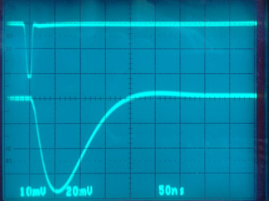
[24-APR-19] We have our first assembled Amplifier-Shaper A2088D. We have U1 = U2 = ERA-3SM, R1-R4 3dB, L3 = 3.3 μH and C9 = 1.0 nF. Looking at the response to a 20-mV 12-ns pulse, We see signs of oscillation on OUT, and gain varies by a factor of two as we touch the circuit board. We replace L2 = 100 nH with L2 = 0.0 nH. The oscillations stop and the gain is stable.

[10-JUN-19] We report on the linearity and dynamic range of the V2 shaper in V2 Shaper-Amplifier Performance.

[26-JUN-19] The A2088D with C8 = 1.0 nF and C7 = 1.0 μF produces a sustained oscillation of 200-300 MHz at its output with amplitude of order 10 mVpp. We remove C8 and the output noise drops to 2 mVpp, with no obvious oscillations. The 1.0 μF ceramic capacitor in place of C7 is the CGA4J3X7R1H105K125AB with self-resonant frequency 5 MHz and equivalent series resistance 1 Ω at 100 MHz.

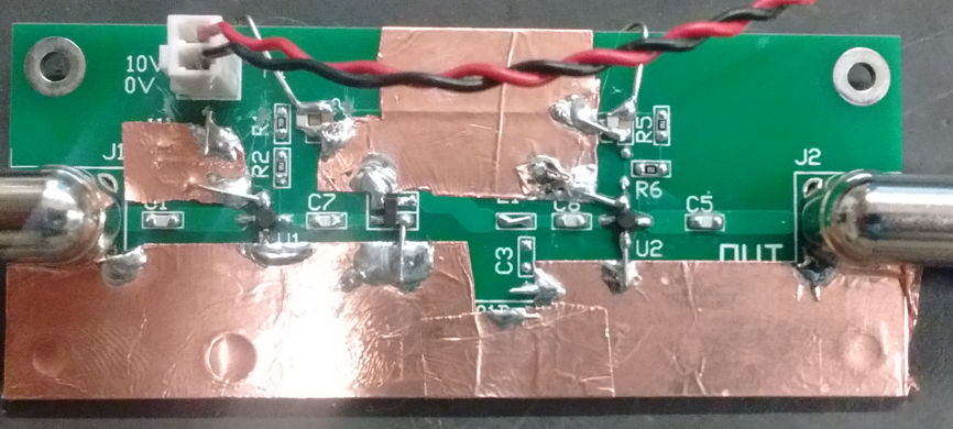
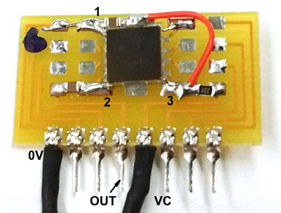
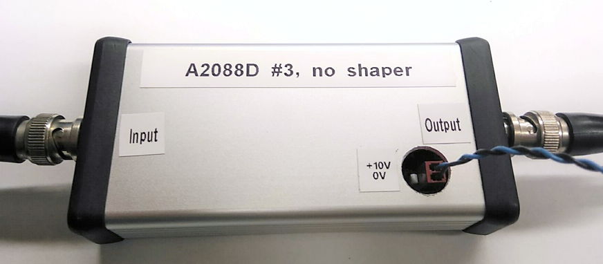
We mount the A2088D in a metal enclosure with plastic end-caps. Note the hole for delivering power with the two-way cable-mounting socket. Connecting the power the wrong way around will not damage the circuit, thanks to diode D1.

We measure gain versus frequency for 10 mVpp sinusoidal input for four A2088D-0 and compare to the ZHL-3A, which should provide flat gain up to 150 MHz. We are using a 300-MHz analog scope to measure output amplitude, and a 160-MHz function generator to provide the input.

Figure: Gain of A2088D-0 with versus Frequency. Measurements by Xinfei Huang.

We apply 12-ns, negative-going pulses to the input. We increase their height and record output pulse height.

Figure: Output Amplitude versus Input Amplitude for A2088D-0. Measurements by Xinfei Huang.

[05-OCT-20] We define the following versions of the A2088D, each named after the length of the pulse it emits for an ideal input pulse of 1 ns. We define pulse width as the time between the pulse rising half-way to its peak and falling half-way from its peak, also known as the Full-Width Half-Height (FWHH).

Our function generator produces pulses of no less than 10 ns. The A2088D-0 reproduces these 10-ns pulses faithfully, as shown below.

Figure: Input and Output of A2088D-0. Left: Pulse from function generator. Right: Pulse from A2088D-0 for input shown on left. (By Xinfei Huang)

We measure gain versus frequency of the A2088D-0, using a 1-m RJ-58C/U cable from a synthesizer, and a spectrometer with 50-Ω input connected directly to the amplifier output. When we connect the synthesizer directly to the spectrometer we see −40±2 dBm. The amplifier output varies by far more.

Figure: Gain of A2088D-0 versus Frequency.

The ERA-3SM amplifier gain is typically 22 dB at 100 MHz, 21 dB at 1 GHz, 19 dB at 2 GHz, and 16 dB at 3 GHz. We have two ERA-3SM and 12 dB of attenuition, so we expect 32 dB at 100 MHz, 30 dB at 1 GHz, 26 dB at 2 GHz and 20 dB at 3 GHz.

SiPM Head, Version Two

[05-MAR-20] We damage three SiPMs by connecting power to them the wrong way around. There is an error in the power plug footprint of the A208801C printed ciruit board, and resistor R1 = 1 kΩ allows 30 mA to flow in the foreward direction through D1 when we connect 30 V to the anode. In the new circuit, we increase R1 to 10 kΩ, eliminate L1, and switch to board-edge right-angle connectors.

Figure: SiPM Head, Version Two, Schematic.

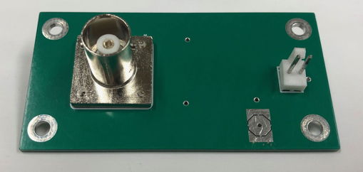
We lay out the A208801E. This board has space to put a 5-cm square scintillator over the SiPM, and holes for standoffs to mount the scintillator. Connectors are on the bottom side, right-angled near the board edge.

Figure: SiPM Head, Version Two, Top Side. The board is two-layer, black solder mask, 0.062" thick, with the ground plane on the bottom layer.

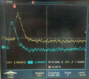
[26-AUG-20] As we report in Silicon Photomultipliers: Characterization and Cosmic Ray Detection, with two SiPM-scintillator combinations, we can detect coincident light pulses generated by cosmic muons. The screen shot below is one such pulse, fed directly into an oscilloscope.

Figure: Muon Hit in 6-mm Square SiPM, Seen Without Amplification on Oscilloscope.

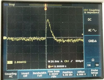
The MICROFC data sheet gives 3.2 ns as the length of a single-photon pulse generated by the 6-mm square SiPM. Our pulse is 20 ns long. We do not know the relaxation time constant of our plastic scintillator, but we expect it to be no more than 4 ns. The pulse we observe here is 20 ns long.

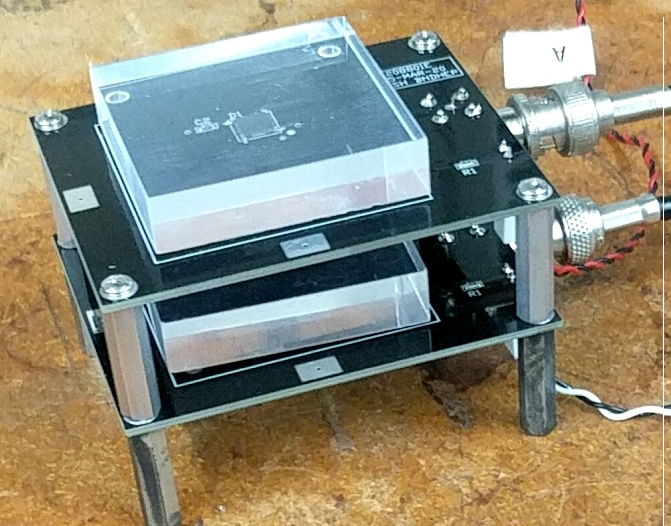
[14-SEP-20] We assemble two SiPM A2088E boards together with their own scintillators.

Figure: Two A2088E SiPM Heads Joined with Scintillators. By Nathan Sayer.

The cable we use to connect the first SiPM to oscilloscope channel No1 is 1.5 m longer than the cable we use to connect the second to channel No2. We observe the following muon pulses in one event.

Figure: Muon Hit in 6-mm Square SiPM, Seen Without Amplification on Oscilloscope. By Nathan Sayer

The No1 pulse is delayed by 8 ns with respect to the No2 pulse, which is consistent with the propagation delay of 1.5 m of coaxial cable.

[02-NOV-20] With two 5-cm square pieces of scintillator and two SiPM detectors arranged as shown above, we measure the frequency of muons passing through both scintillators by counting simultaneous pulses on the oscilloscope. We have the two scintillators aligned parallel with their centers on a common perpendicular. We align this perpendicular vertically and obtain roughly one hit per minute. We rotate from the vertical and obtain the following plot.

Figure: Muon Hit Rate Variation with Angle from Vertical for Two 5-cm Scintillator Squares 5 cm Apart and Parallel. By Nathan Sayer

We have an LED coupled to an optical fiber. We bring the fiber into our dark box and shine its light upon a bare SiPM. We reduce the intensity of the LED by increasing a series resistor. We flash the LED for 25 ns. Our LED driver board provides a post-flash trigger that we can use with our digital storage oscilloscope to capture the output of the SiPM during the light pulse. When the light is dim enough, we sometimes see no pulse, and sometimes one pulse. As we brighten the pulse, we will sometimes see two pulses. Assuming each pulse is a photon, we make the following histogram.

Figure: Photon Frequency During Dim Light Pulse. We see zero, one, or two pulses from the SiPM, with distribution that depends upon the value of the LED's series resistor. By Nathan Sayer

[04-JAN-21] We have a Python simulation of pulse shapers prepared by Xinfei Huang, shaper_sim.py. Define the inductor, capacitor, pulse length, and resistances with an file input.txt like this:

Note: This txt file will be read when shaper_sim.py is executed. The script read off parameters from this file. 

Note: Use single space to separate values. 
L (uH): .1 1 3.3 4.7 6.8 10 27
C (nF): .0033 .015 .033 .047 .1 .27 1

input pulse duration (ns): 15

R1 (Ohm): 50
R2 (Ohm): 50

Then run with "python3 shaper_sim.py" on MacOS, or equivalent command on your operating system. The program creats a folder Plots that contains plots of the pulse shape for all combinations of the above inductor and capacitor values.

[06-JUN-21] We measure dark current versus temperature.

Figure: Dark Current Versus Temperature. By Nathan Sayer

[06-AUG-21] A comparison of measured and simulated muon hit rate, using data from earlier this year.

Figure: Simulated and Measured Hit Rate, Normalized with respect to Vertical. By Nathan Sayer